Machine Learning Crash Course
COS 351 - Computer Vision
recap: multiple views and motion
- Epipolar Geometry
- Relates cameras in two positions
- Fundamental matrix maps from a point in one image to a line (its epipolar line) in the other
- Can solve for \(F\) given corresponding points (e.g., interest points)
- Stereo Depth Estimation
- Estimate disparity by finding corresponding points along epipolar lines
- Depth is inverse to disparity
recap: multiple views and motion
- Motion Estimation
- By assuming brightness constancy, truncated Taylor expansion leads to simple and fast patch matching across frames
- Assume local motion is coherent
- "Aperture problem" is resolved by coarse to fine approach
\[\nabla I \cdot \left[\begin{array}{cc} u & v \end{array}\right]^T + I_t = 0\]
Structure from motion (or SLAM)
Given a set of corresponding points in two or more images, compute the camera parameters and the 3D point coordinates
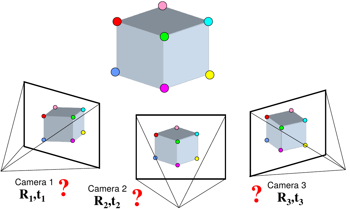
Structure from motion (or SLAM)
structure from motion ambiguity
If we scale the entire scene by some factor \(k\) and, at the same time, scale the camera matrices by the factor of \(1/k\), the projections of the scene points in the image remain exactly the same:
\[\mathbf{x} = \mathbf{P}\mathbf{X} = \left(\frac{1}{k} \mathbf{P}\right)(k\mathbf{X})\]
It is impossible to recover the absolute scale of the scene!
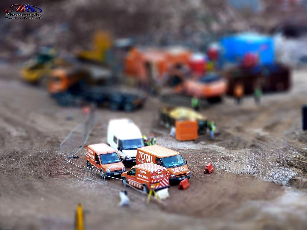
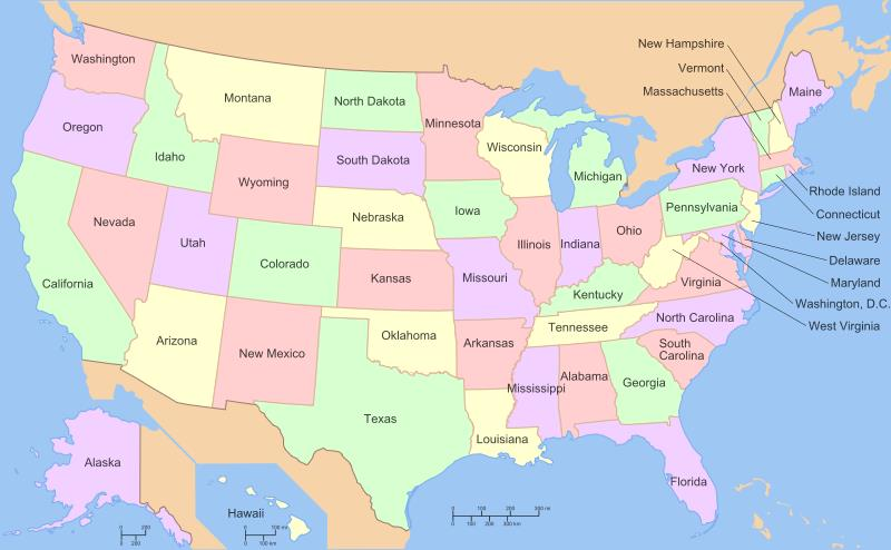
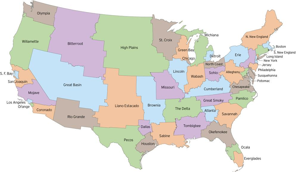
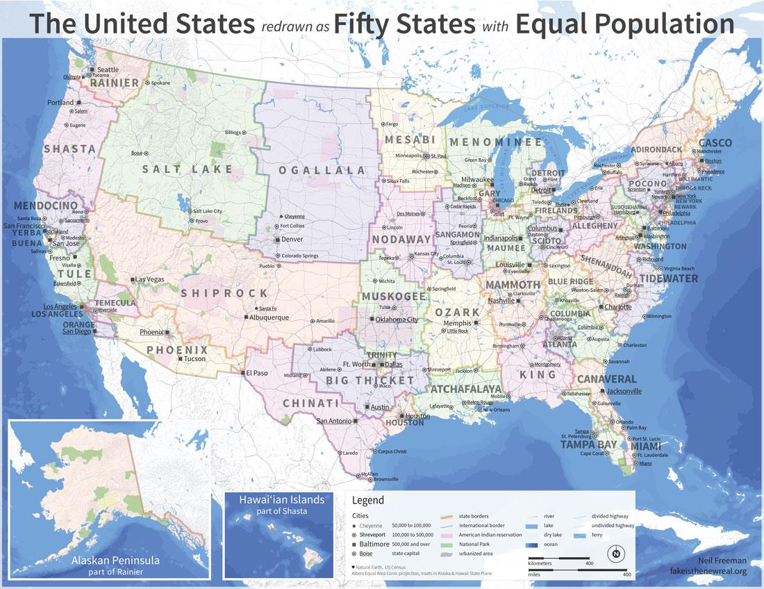
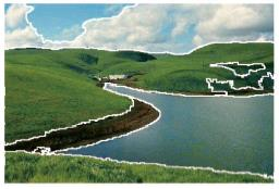
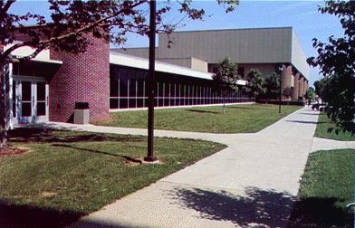
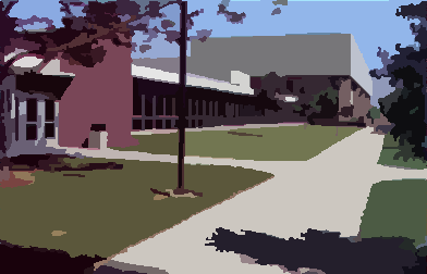
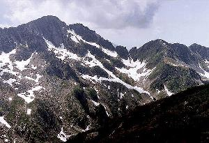
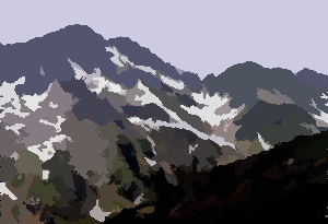
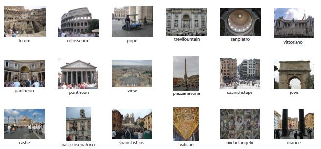
what is the scale of image content?
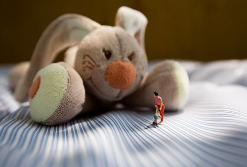
what is the scale of image content?
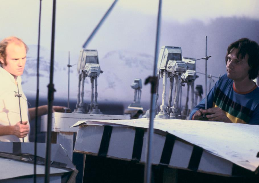
what is the scale of image content?
bundle adjustment
- Non-linear method for refining structure and motion
- Minimizing reprojection error
\[E(\mathbf{P}, \mathbf{X}) = \sum_{i=1}^m \sum_{j=1}^n D\left(\mathbf{x}_{ij}, \mathbf{P}_i \mathbf{X}_j\right)^2\]
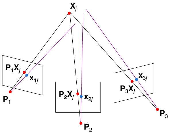
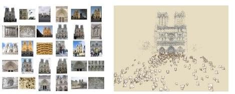
photo synth
Noah Snavely, Steven M. Seitz, Richard Szeliski. Photo tourism: Exploring photo collections in 3D. SIGGRAPH 2006
machine learning: overview
- Core of ML: Making predictions or decisions from data
- This overview will not go into depth about the statistical underpinnings of learning methods. We're looking at ML as a tool.
- Take a machine learning course if you want to know more!
(COS 280, SYS 411)
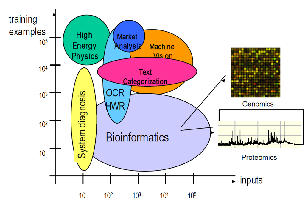
impact of machine learning
Machine Learning is arguably the greatest export from computing to other scientific fields
machine learning applications
machine learning problems
| supervised learning |
unsupervised learning | |
|---|---|---|
| discrete | classification or categorization | clustering |
| continuous | regression | dimensionality reduction |
machine learning problems
| supervised learning |
unsupervised learning | |
|---|---|---|
| discrete | classification or categorization | clustering |
| continuous | regression | dimensionality reduction |
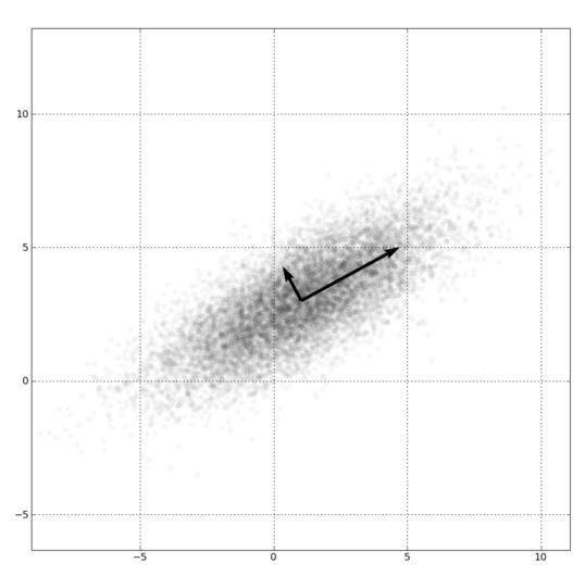
dimensionality reduction
|
 |
machine learning problems
| supervised learning |
unsupervised learning | |
|---|---|---|
| discrete | classification or categorization | clustering |
| continuous | regression | dimensionality reduction |
clustering
clustering
clustering
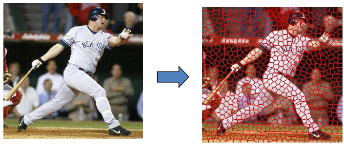
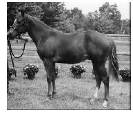
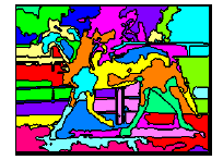
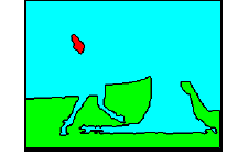
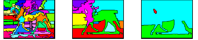
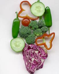
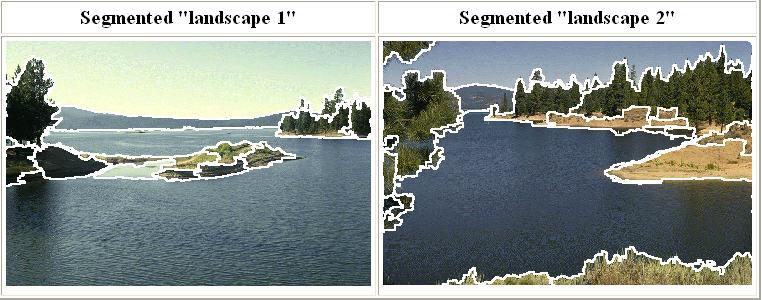
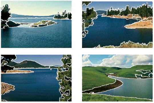
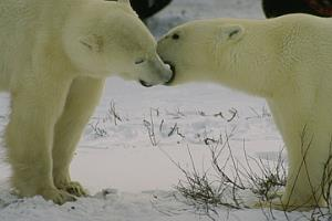
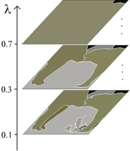
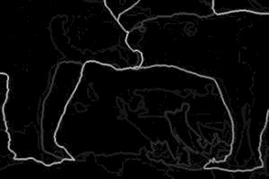
clustering example: image segmentation
Goal: break up the image into meaningful or perceptually similar regions
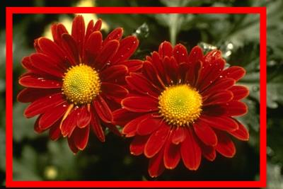
segmentation for feature support or efficiency
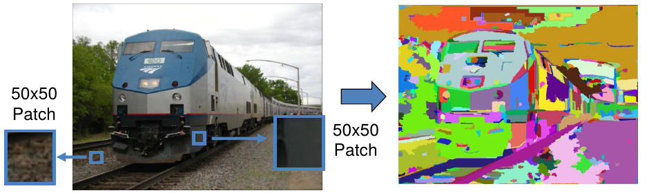
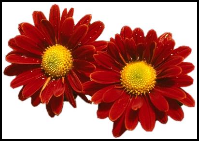
segmentation as a result
types of segmentation
clustering
- Clustering
- group together similar points and represent them with a single token
Key challenges
- What makes two points/images/patches similar?
- How do we compute an overall grouping from pairwise similarities?
why do we cluster?
- Summarizing data
- Look at large amounts of data
- Patch-based compression or denoising
- Represent a large continuous vector with the cluster number
- Counting
- Histograms of texture, color, SIFT vectors
- Segmentation
- Separate the image into different regions
- Prediction
- Images in the same cluster may have the same labels
how do we cluster?
- K-means
- Iteratively re-assign points to the nearest cluster center
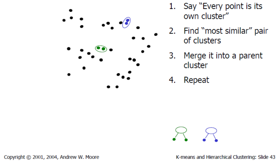
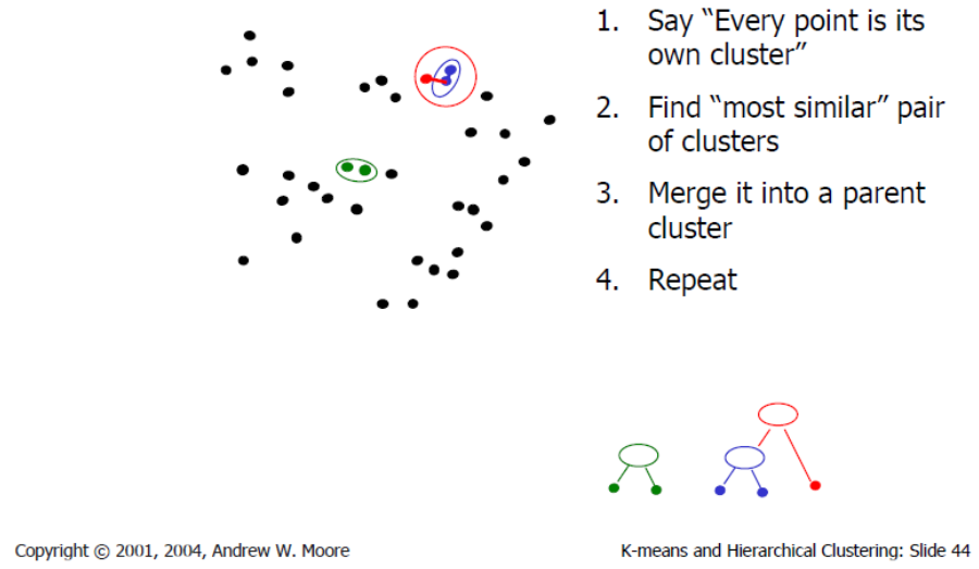
- Agglomerative clustering
- Start with each point as its own cluster and iteratively merge the closest clusters
- Mean-shift clustering
- Estimate modes of PDF
- Spectral clustering
- Split the nodes in a graph based on assigned links with similarity weights
clustering for summarization
Goal: cluster to minimize variance in data given clusters
- Preserve information
\[\mathbf{c}^*, \mathbf{\delta}^* = \argmin{\mathbf{c},\mathbf{\delta}} \frac{1}{N} \sum_j^N \sum_i^K \delta_{ij} \left( \mathbf{c}_i - \mathbf{x}_j \right)^2\]
\(\mathbf{c}_i\): cluster center
\(\mathbf{x}_j\): data
\(\delta_{ij}\): whether \(\mathbf{x}_j\) is assigned to \(\mathbf{c}_i\)
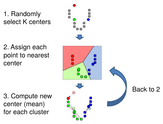
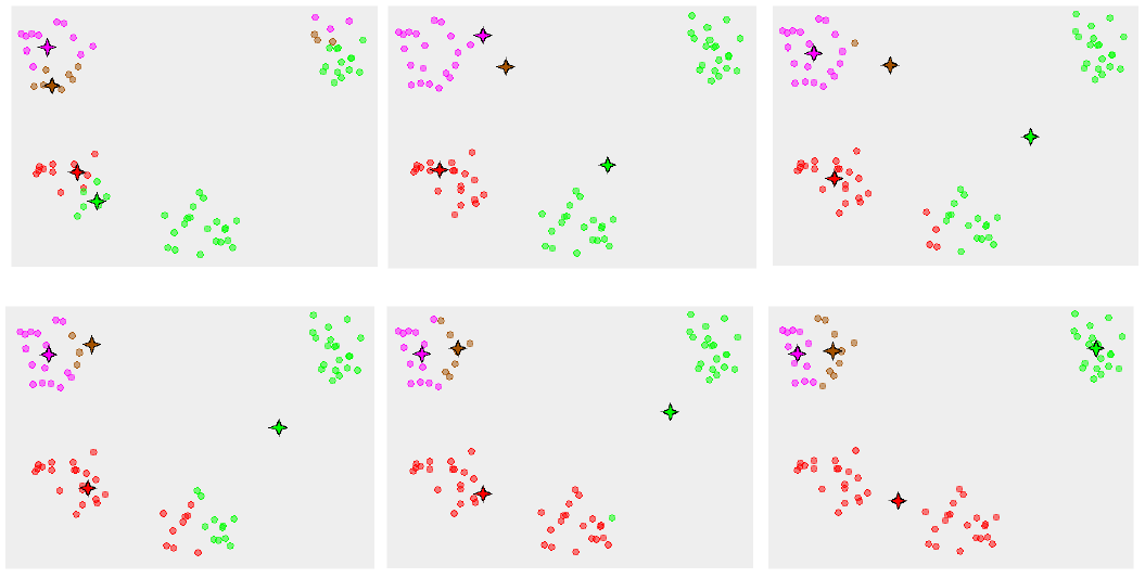
K-means algorithm

K-means algorithm
K-means algorithm
- Initialize cluster centers: \(\mathbf{c}^0\); \(t=0\)
- Assign each point to the closest center \[\mathbf{\delta}^t = \argmin{\mathbf{\delta}} \frac{1}{N} \sum_j^N \sum_i^K \delta_{ij}^{t-1} \left( \mathbf{c}_i^{t-1} - \mathbf{x}_j \right)^2\]
- Update cluster centers as the mean of the points \[\mathbf{c}^t = \argmin{\mathbf{c}} \frac{1}{N} \sum_j^N \sum_i^K \delta_{ij}^{t-1} \left( \mathbf{c}_i^{t-1} - \mathbf{x}_j \right)^2\]
- Repeat 2–3 until no points are re-assigned (\(t=t+1\))
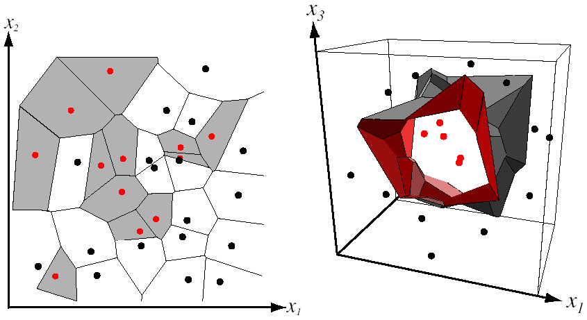
k-means converges to a local minimum
k-means: design choices
- Initialization
- Randomly select \(K\) points as initial cluster center
- Or greedily choose \(K\) points to minimize residual
- Distance measures
- Traditionally Euclidean, could be others
- Optimization
- Will converge to a local minimum
- May want to perform multiple restarts
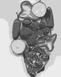
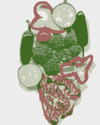
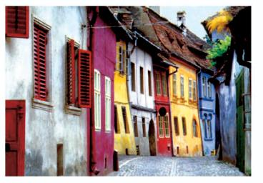
k-means clustering using intensity or color
how to evaluate clusters?
- Generative
- How well are points reconstructed from the clusters?
- Discriminative
- How well do the clusters correspond to labels?
- Purity
- Note: unsupervised clustering does not aim to be discriminative
- How well do the clusters correspond to labels?
how to choose the number of clusters?
- Validation set
- Try different numbers of clusters and look at performance
- When building dictionaries (discussed later), more cluster typically work better
- Try different numbers of clusters and look at performance
k-means pros and cons
- Pros
- Finds cluster centers that minimize conditional variance (good representation of data)
- Simple and fast*
- Easy to implement
k-means pros and cons
- Pros
- Cons
- Need to choose \(K\)
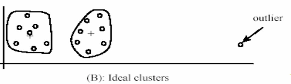
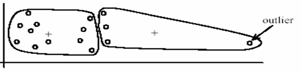
- Sensitive to outliers
- Prone to local minima
- All clusters have the same parameters (e.g., distance measure is non-adaptive)
- *Can be slow: each iteration is \(O(KNd)\) for \(N\) \(d\)-dimensional points
k-means pros and cons
- Pros
- Cons
- Usage
- Rarely used for pixel segmentation
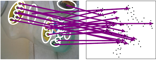
building visual dictionaries
- Sample patches from a database
- e.g., 128 dimensional SIFT vectors
- Cluster the patches
- Cluster centers are the dictionary
- Assign a codeword (number) to each new patch according to the nearest cluster
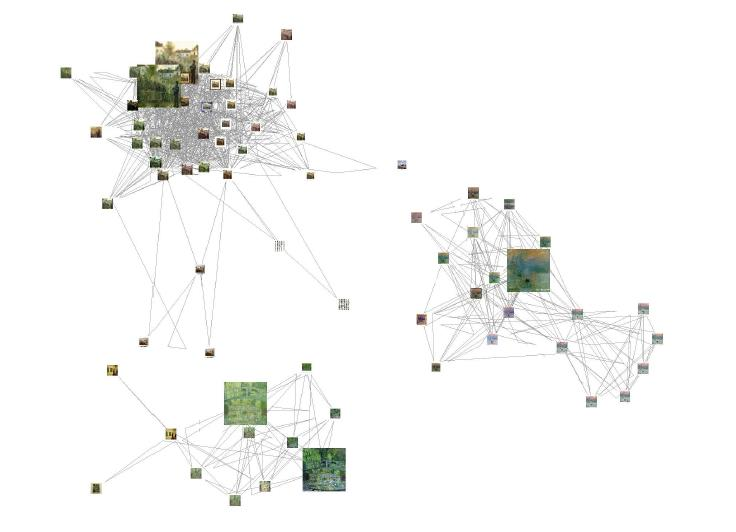
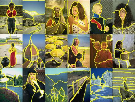
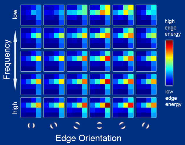
examples of learned codewords
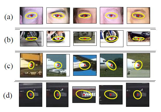
Most likely codewords for 4 learned "topics"
EM with multinomial (problem 3) to get topics
agglomerative clustering
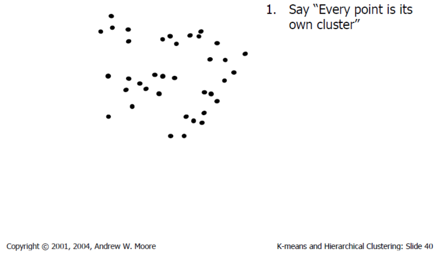
agglomerative clustering
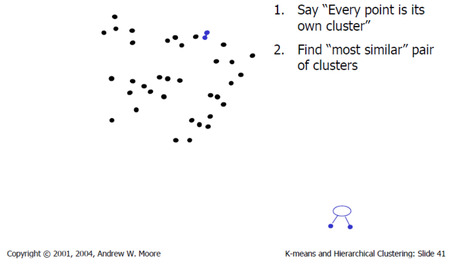
agglomerative clustering
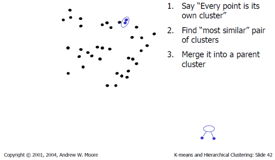
agglomerative clustering
agglomerative clustering
agglomerative clustering
How to define cluster similarity?
- Average distance between points, maximum distance, minimum distance
- Distance between means or mediods
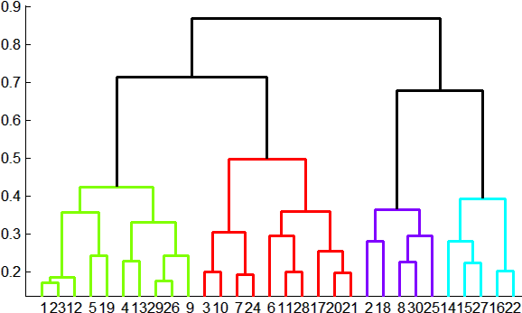
How many clusters?
- Clustering creates a dendrogram (a tree)
- Threshold based on max number of clusters or based on distance between merges
conclusions: agglomerative clustering
- Pros
- Simple to implement, widespread application
- Clusters have adaptive shapes
- Provides a hierarchy of clusters
- Cons
- May have imbalanced clusters
- Still have to choose number of clusters or threshold
- Need to use an "ultrametric" to get a meaningful hierarchy
mean shift segmentation
Mean shift segmentation is a versatile technique for clustering-based segmentation
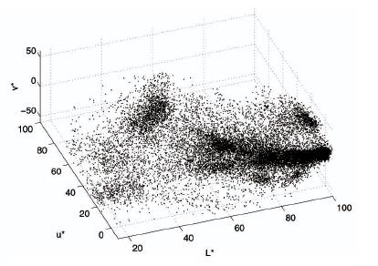
mean shift algorithm
Try to find modes of this non-parametric density
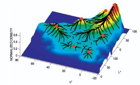
kernel density estimation
Kernel density estimation
\[\hat{f}_h(x) = \frac{1}{nh} \sum_{i=1}^n K \left( \frac{x-x_i}{h} \right)\]
Gaussian kernel
\[K \left( \frac{x-x_i}{h} \right) = \frac{1}{\sqrt{2\pi}} e^{-\frac{(x-x_i)^2}{2h^2}}\]
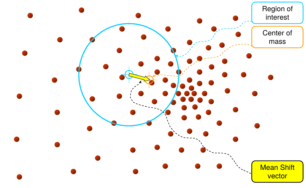
mean shift
mean shift

mean shift
mean shift
mean shift

mean shift
mean shift
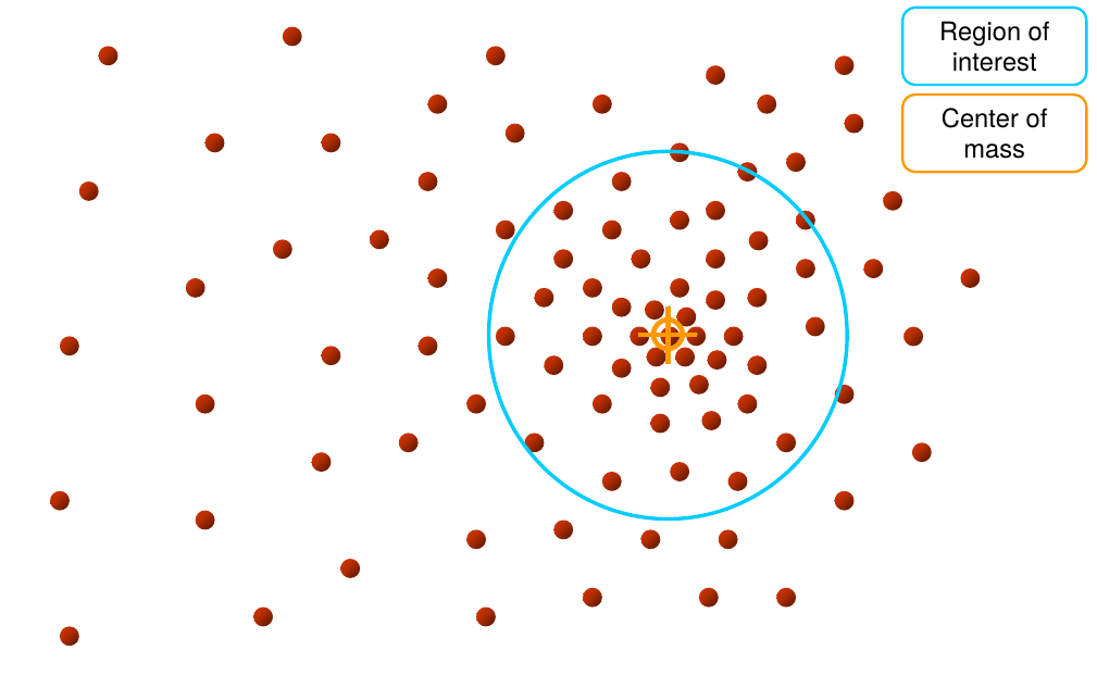
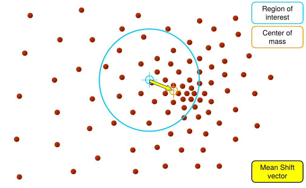
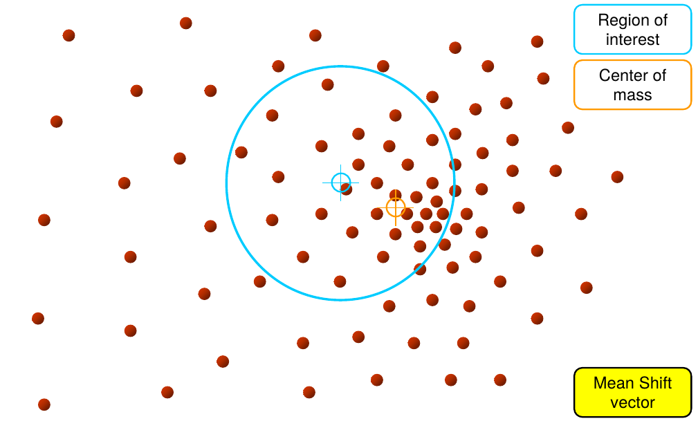
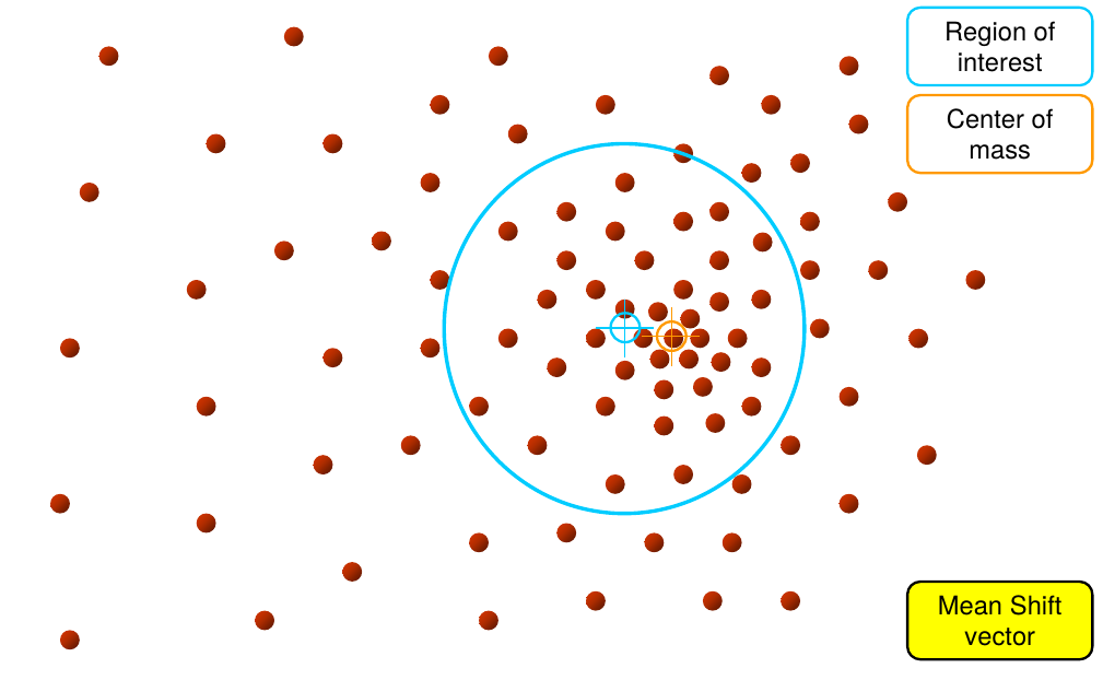
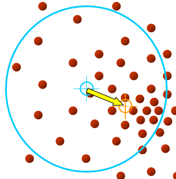
computing the mean shift
Simple mean shift procedure
- Compute mean shift vector
- Translate the kernel window by \(\mathbf{m}(\mathbf{x})\)
|
\[\mathbf{m}(\mathbf{x}) = \left[ \frac{\sum_{i=1}^n \mathbf{x}_i g\left( \frac{||\mathbf{x} - \mathbf{x}_i||^2}{h} \right)}{\sum_{i=1}^n g\left( \frac{||\mathbf{x}-\mathbf{x}_i||^2}{h} \right)} - \mathbf{x} \right]\] \(\mathbf{x}\): current location (cyan cross) |
 |
attraction basin
- Attraction Basin
- the region for which all trajectories lead to the same mode
- Cluster
- all data points in the attraction basin of a mode
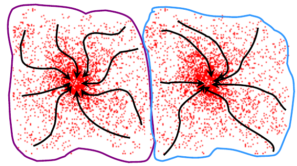
attraction basin
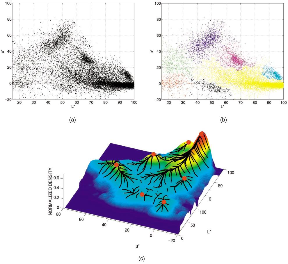
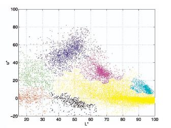
mean shift clustering
The mean shift algorithm seeks modes of the given set of points
- Choose kernel and bandwidth
- For each point
- Center a window on that point
- Compute the mean of the data in the search window
- Center the search window at the new mean location
- Repeat 2–3 until convergence
- Assign points that lead to nearby modes to the same cluster
segmentation by means shift
- Compute features for each pixel (color, gradients, texture, etc.)
- Set kernel size for features \(K_f\) and position \(K_s\)
- Initialize windows at individual pixel locations
- Perform mean shift for each window until convergence
- Merge windows that are within width of \(K_f\) and \(K_s\)
mean shift segmentation results
mean shift segmentation results
mean shift pros and cons
- Pros
- Good general-practice segmentation
- Flexible in number and shape of regions
- Robust to outliers
- Cons
- Have to choose kernel size in advance
- Not suitable for high-dimensional features
- When to use it
- Oversegmentation
- Multiple segmentations
- Tracking, clustering, filtering applications
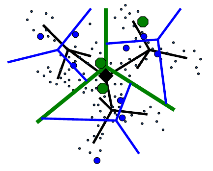
spectral clustering
Group points based on links in a graph
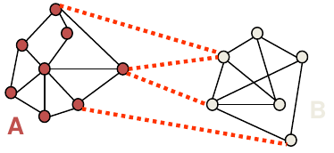
cuts in a graph
Normalized cut
- a cut penalizes large segments
- fix by normalizing for size of segments \[\mathit{Ncut}(A,B) = \frac{\mathit{cut}(A,B)}{\mathit{volume}(A)} + \frac{\mathit{cut}(A,B)}{\mathit{volume}(B)}\]
- \(\mathit{volume}(A) = \text{sum of costs of all edges that touch }A\)
normalized cuts for segmentation
which algorithm to use?
- Quantization / Summarization: K-means
- aims to preserve variance of original data
- can easily assign new point to a cluster
|
|
|

which algorithm to use?
- Image segmentation: Agglomerative clustering
- More flexibile with distance measures (e.g., can be based on boundary prediction)
- Adapts better to specific data
- Hierarchy can be useful
clustering
Key algorithm: K-means
machine learning problems
| supervised learning |
unsupervised learning | |
|---|---|---|
| discrete | classification or categorization | clustering |
| continuous | regression | dimensionality reduction |
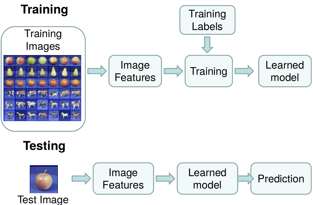
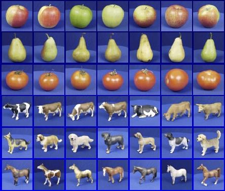
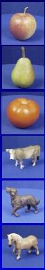
the machine learning framework
Apply a prediction function (\(f\)) to a feature representation of the image (input) to get the desired output:
- \(f\Bigl(\)
 \(\Bigr) \Rightarrow \text{"apple"}\)
 - \(f\Bigl(\)
 \(\Bigr) \Rightarrow \text{"tomato"}\)
 - \(f\Bigl(\)
 \(\Bigr) \Rightarrow \text{"cow"}\)
the machine learning framework
\[y = f(\mathbf{x})\]
\(y\): output
\(f\): prediction function
\(\mathbf{x}\): image feature
- Training: given a training set of labeled examples \(\{(\mathbf{x}_1,y_1, \ldots, (\mathbf{x}_N, y_N)\}\), estimate the prediction function \(f\) by minimizing the prediction error on the training set
- Testing: apply \(f\) to a never before seen test example \(\mathbf{x}\) and output the predicted value \(y = f(\mathbf{x})\)
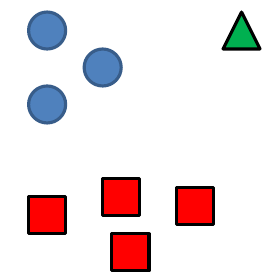
learning a classifier
Given some set of features with corresponding labels, learn a function to predict the labels from the features
learning a classifier
Given some set of features with corresponding labels, learn a function to predict the labels from the features
learning a classifier
Given some set of features with corresponding labels, learn a function to predict the labels from the features
steps
features
- Raw pixels
- Histograms
- GIST descriptors
- ...
one way to think about it
- Training labels dictate that two examples are the same or different, in some sense
- Features and distance measures define visual similarity
- Classifiers try to learn weights or parameters for features and distance measures so that visual similarity predicts label similarity
many classifiers to choose from
- SVM
- Neural networks
- Naive Bayse
- Bayesian network
- Logistic regression
- Randomized Forests
- Boosted Decision Trees
- K-Nearest Neighbors
- RBMs
- etc.
Which one is best?
Claim:
The decision to use machine learning is more important than the choice of a particular learning method
Classifiers: Nearest neighbors
\[f(\mathbf{x}) = \text{label of the training example nearest to }\mathbf{x}\]
- All we need is a distance function for our inputs
- No training required!
Classifiers: Linear
\[f(\mathbf{x}) = \mathit{sgn}(\mathbf{w} \cdot \mathbf{x} + b)\]
- Find a linear function to separate the classes
recognition task and supervision
- Images in the training set must be annotated with the "correct answer" that the model is expected to produce
spectrum of supervision
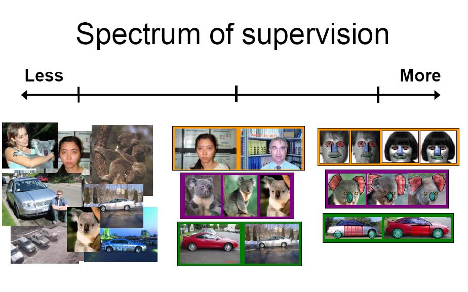
| Unsupervised | "Weakly" Supervised | Fully Supervised |
Weakly vs Fully: definition depends on task
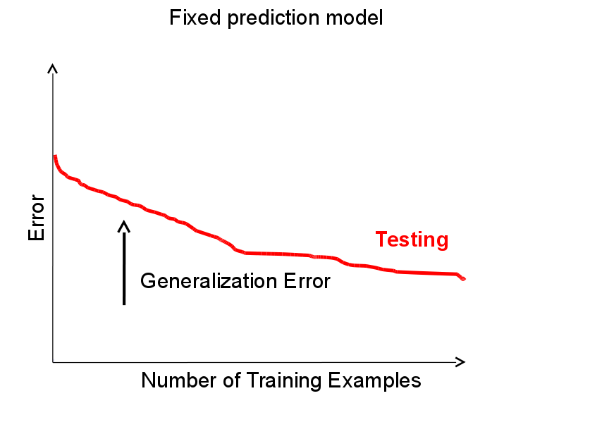
generalization
How well does a learned model generalize from the data it was trained on to a new test set?
generalization
- Components of generalization error
- Bias: how much the average model over all training sets differ from the true model?
- Error due to inaccurate assumptions/simplifications made by the model
- Variance: how much models estimated from different training sets differ from each other
- Bias: how much the average model over all training sets differ from the true model?
- ...
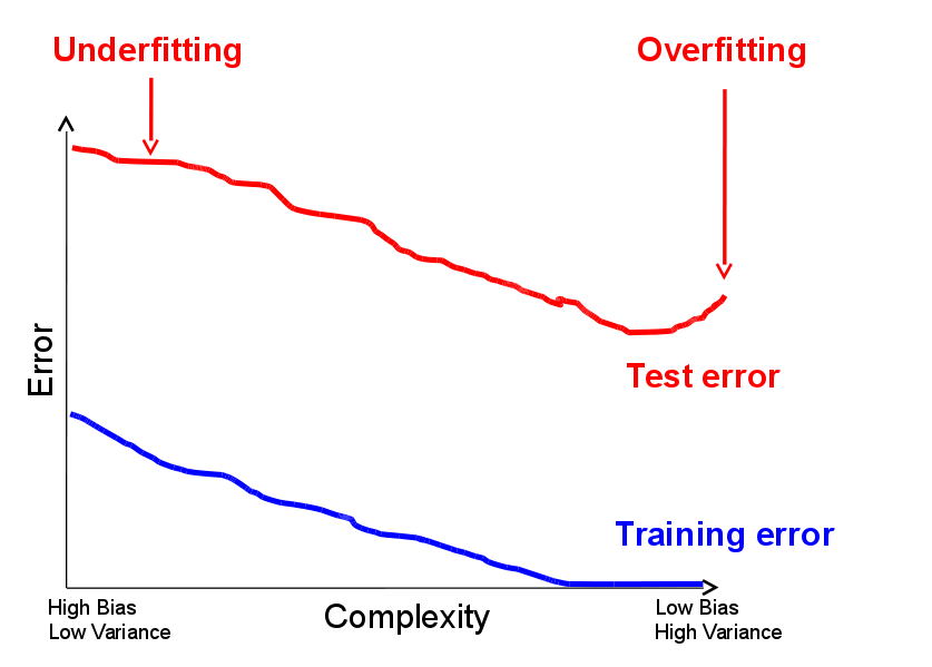
generalization
- Components of generalization error
- Underfitting: model is too "simple" to represent all the relevant class characteristics
- High bias (few degrees of freedom) and low variance
- High training error and high test error
- ...
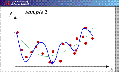
generalization
- Components of generalization error
- Underfitting: model is too "simple" to represent all the relevant class characteristics
- Overfitting: model is too "complex" and fits irrelevant characteristics (noise) in the data
- Low bias (many degrees of freedom) and high variance
- Low training error and high test error
bias-variance trade off
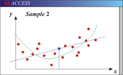
- Models with too few parameters are inaccurate because of a large bias (not enough flexibility)
- Models with too many parameters are inaccurate because of a large variance (too much sensitivity to the sample)
bias-variance trade off
\[E(MSE) = \text{noise}^2 + \text{bias}^2 + \text{variance}\]
\(\text{noise}\): Unavoidable Error
\(\text{bias}\): Error due to incorrect assumptions
\(\text{variance}\): Error due to variance of training samples
See link for explanations of bias-variance (also Bishop's "Neural Networks" book)
bias-variance trade off
bias-variance trade off
bias-variance trade off
remember...
No classifier is inherently better than any other; you need to make assumptions to generalize
Three kinds of error:
- Inherent: unavoidable
- Bias: due to over-simplifications
- Variance: due to inability to perfectly estimate parameters from limited data
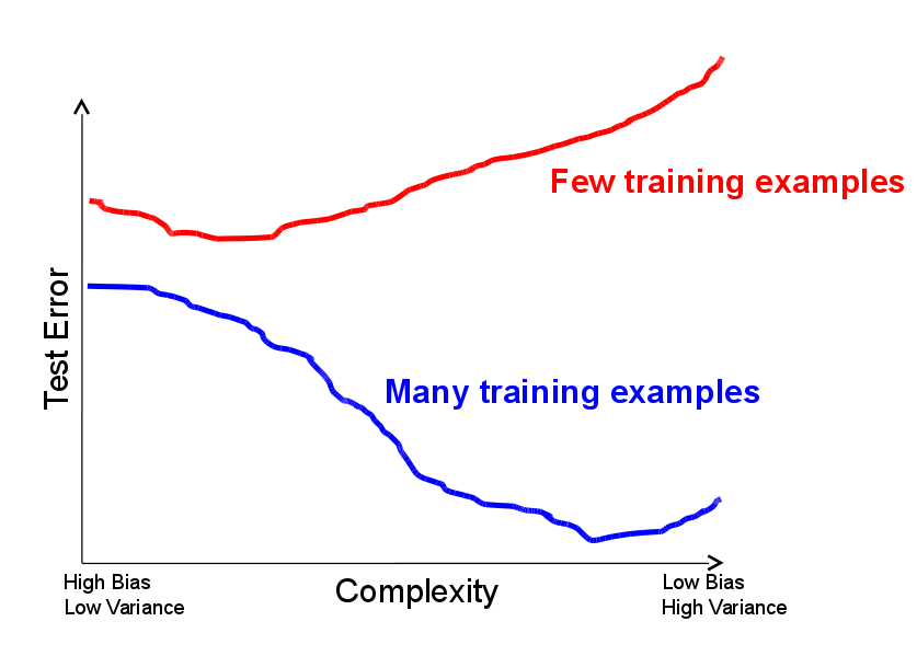
how to reduce variance?
Ways to reduce variance
- Choose a simpler classifier
- Regularize the parameters
- Get more training data
very brief tour of some classifiers
- K-nearest neighbors
- SVM
- Boosted Decision Trees
- Neural networks
- Naive Bayes
- Bayesian network
- Logistic regression
- Randomized forests
- RBMs
- etc.
generative vs. discriminative classifiers
|
Generative Models
|
Discriminative Models
|
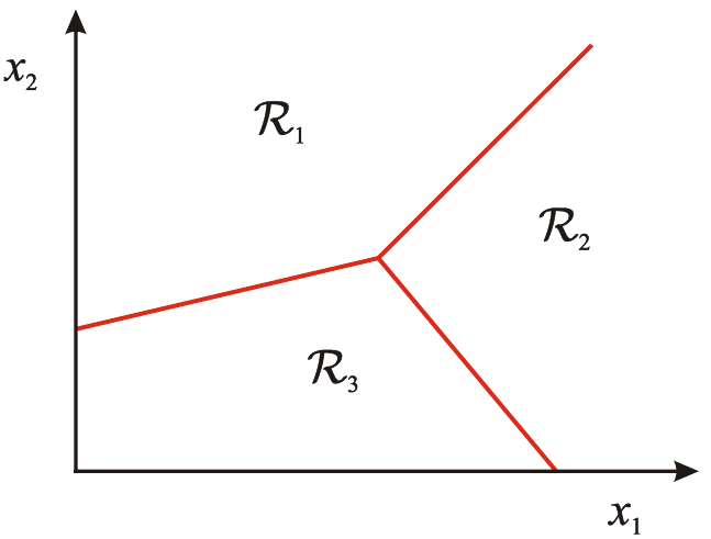
classification
Assign input vector to one of two or more classes
Any decision rule divides input space into decision regions sepearated by decision boundaries
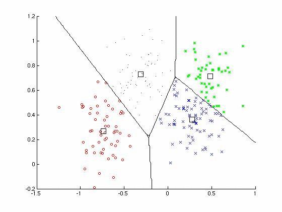
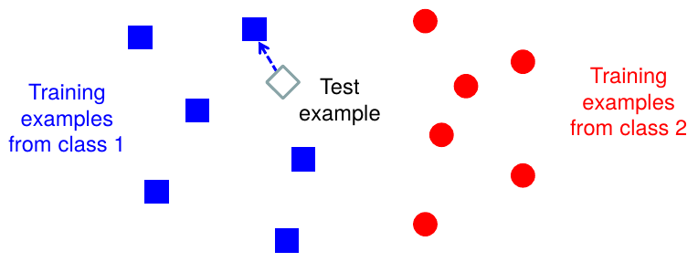
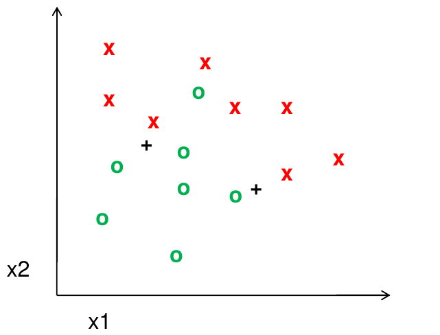
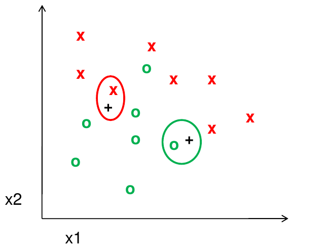
classifiers: k-nearest neighbor
Assign label of nearest training data point to each test data point
classifiers: k-nearest neighbor
classifiers: k-nearest neighbor
classifiers: k-nearest neighbor
classifiers: k-nearest neighbor
classifiers: k-nearest neighbor
Using k-NN
- Simple, a good one to try first
- With infinite examples, 1-NN provably has error that is at most twice Bayes optimal error
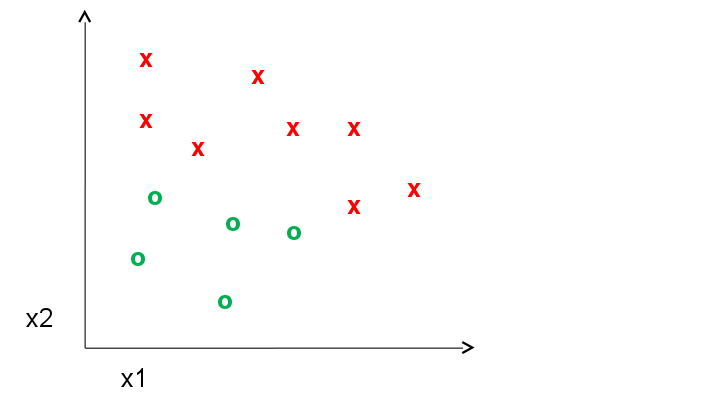
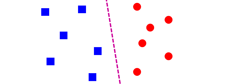
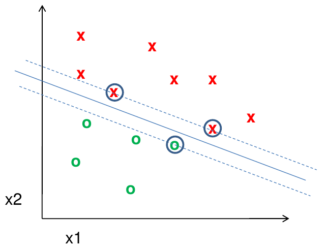
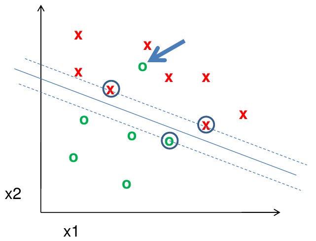
classifiers: Linear SVM
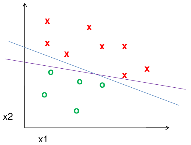
Find a linear function to separate the classes:
\[f(\mathbf{x}) = \mathrm{sgn}(\mathbf{w}\cdot\mathbf{x} + b)\]
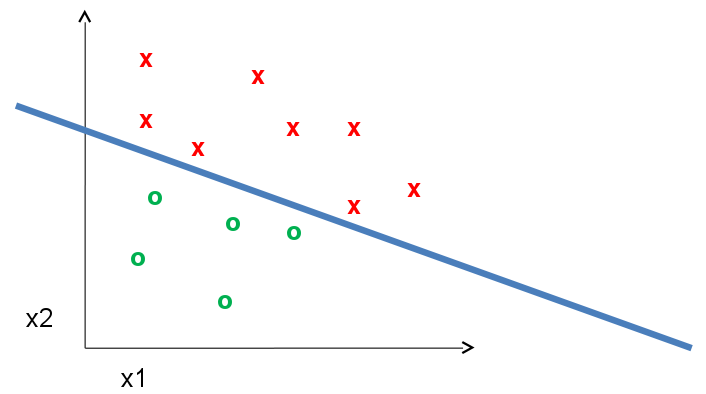
classifiers: Linear SVM
Find a linear function to separate the classes:
\[f(\mathbf{x}) = \mathrm{sgn}(\mathbf{w}\cdot\mathbf{x} + b)\]
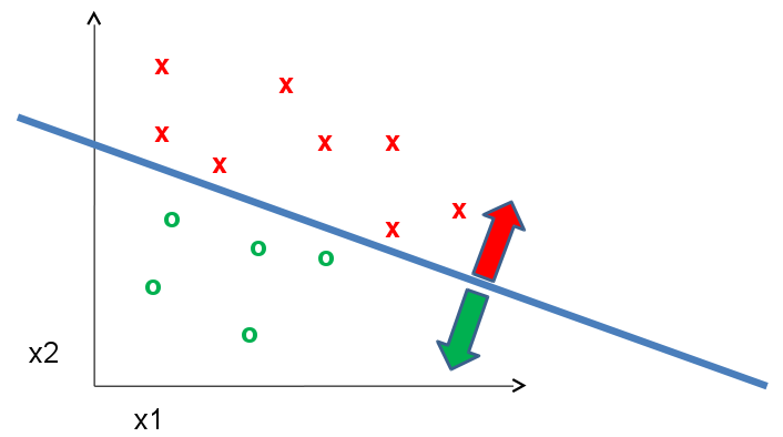
classifiers: Linear SVM
Find a linear function to separate the classes:
\[f(\mathbf{x}) = \mathrm{sgn}(\mathbf{w}\cdot\mathbf{x} + b)\]
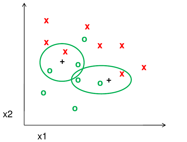
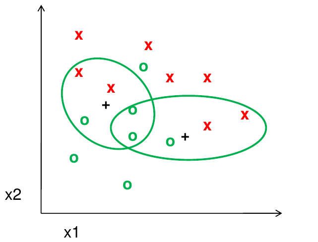
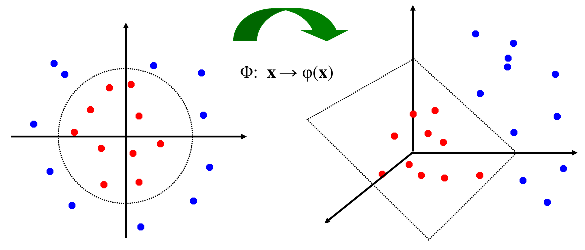
classifiers: nonlinear SVMs
Datasets that are linearly separable work out great
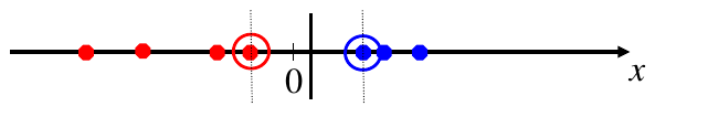
But what if the dataset is just too hard?
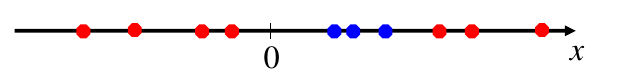
We can map it to a higher-dimensional space!
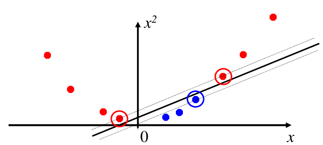
classifiers: nonlinear SVMs
General idea: the original input space can always be mapped to some higher-dimensional feature space where the training set is separable.
classifiers: nonlinear SVMs
The Kernel Trick: instead of explicitly computing the lifting transformation \(\varphi(\mathbf{x})\), define a kernel function \(K\) such that
\[K(\mathbf{x}_i, \mathbf{x}_j) = \varphi(\mathbf{x}_i)\cdot\varphi(\mathbf{x}_j)\]
Note: to be valid, the kernel function must satisfy Mercer's condition
This gives a nonlinear decision boundary in the original feature space
\[\sum_i \alpha_i y_i \varphi(\mathbf{x}_i) \cdot \varphi(\mathbf{x}) + b = \sum_i \alpha_i y_i K(\mathbf{x}_i, \mathbf{x}) + b\]
C.Burges. A Tutorial on Support Vector Machines for Pattern Recognition. Data Mining and Knowledge Discovery. 1988. link
classifiers: nonlinear SVMs
Example: consider the mapping \(\varphi(x) = (x, x^2)\)
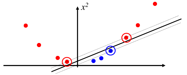
\[\varphi(x) \cdot \varphi(y) = (x, x^2) \cdot (y, y^2) = xy + x^2y+2\] \[ K(x,y) = xy + x^2y^2 \]
Kernel for bags of features
Histogram intersection kernel:
\[I(h_1,h_2) = \sum_{i=1}^N \min(h_1(i), h_2(i))\]
Generalized Gaussian kernel:
\[K(h_1, h_2) = \exp\left( -\frac{1}{A} D(h_1, h_2)^2 \right)\]
\(D\) can be (inverse) L1 distance, Euclidean distance, \(\chi^2\) distance, etc.
J.Zhang, M.Marszalek, S.Lazebnik, C.Schmid. Local Features and Kernels for Classification of Texture and Object Categories: A Comprehensive Study. IJCV 2007. link
summary: SVMs for image classification
- Pick an image representation (in our case, bag of features)
- Pick a kernel function for that representation
- Compute the matrix of kernel values between every pair of training examples
- Feed the kernel matrix into your favorite SVM solver to obtain support vectors and weights
- At test time: compute kernel values for your test example and each support vector, and combine them with the learned weights to get the value of the decision function
what about multi-class SVMs?
- Unfortunately, there is no "definitive" multi-class SVM formulation
- In practice, we have to obtain a multi-class SVM by combining multiple two-class SVMs
- One vs. Others
- Training: learn an SVM for each class vs. the others
- Testing: apply each SVM to test example and assign to it the class of the SVM that returns the highest decision value
- One vs. One
- Training: learn an SVM for each pair of classes
- Testing: each learned SVM "votes" for a class to assign to the test example
SVMs: Pros and Cons
- Pros
- Many publicly available SVM packages. link
- Kernel-based framework is very powerful, flexible
- SVMs work very well in practice, even with very small training sample sizes
- Cons
- No "direct" multi-class SVM, must combine two-class SVMs
- Computation, memory
- During training time, must compute matrix of kernel values for every pair of examples
- Learning can take a very long time for large-scale problems
what to remember about classifiers
- No free lunch: machine learning algorithms are tools, not dogmas
- Try simple classifiers first
- Better to have smart features and simple classifiers than simple features and smart classifiers
- Use increasingly powerful classifiers with more training data (bias-variance tradeoff)
making decisions about data
- 3 important design decisions:
- What data do I use?
- How do I represent my data (what features)?
- What classifier/regressor/machine learning tool do I use?
- These are in decreasing order of importance
- Deep Learning addresses 2 and 3 simultaneously (and blurs the boundary between them)
- You can take the representation from deep learning and use it with any classifier