Motion and Optic Flow
COS 351 - Computer Vision
video
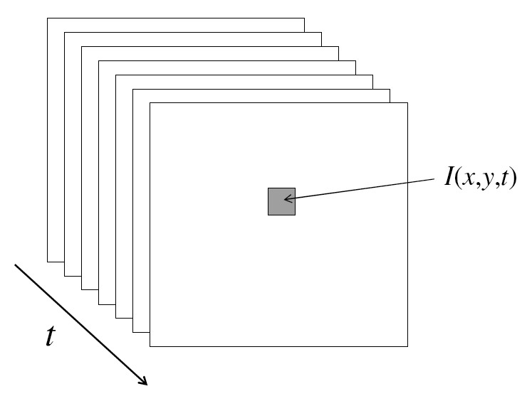
A video is a sequence of frames captured over time
Now our image data is a function of space (\(x,y\)) and time (\(t\)).
motion applications: segmentation of video
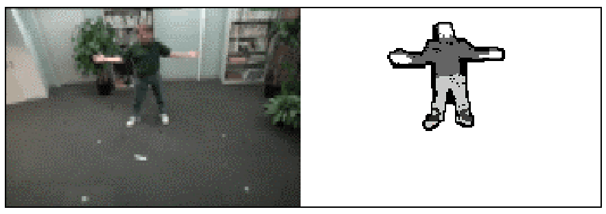
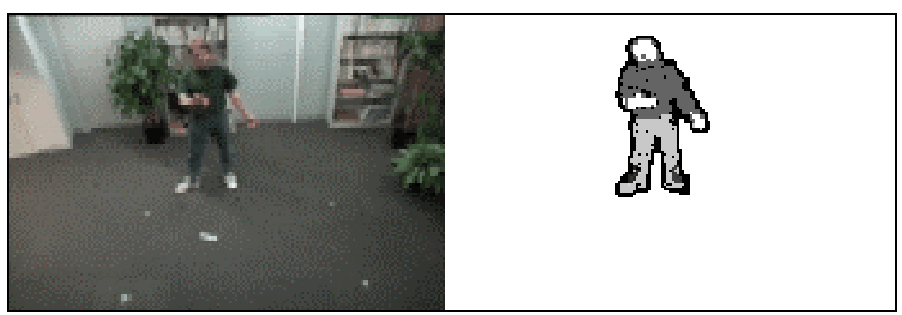
- Background Subtraction
- A static camera is observing a scene
- Goal: separate the static background from the moving foreground
motion applications: segmentation of video
- Background Subtraction
- Shot Boundary Detection
- Commercial video is usually composed of shots or sequences showing the same objects or scene
- Goal: segment video into shots for summarization and browsing (each shot can be represented by a single keyframe in a user interface)
- Difference from background subtraction: the camera is not necessarily stationary

motion applications: segmentation of video
- Background Subtraction
- Shot Boundary Detection
- Motion Segmentation
- Segment the video into multiple coherently moving objects

motion and perceptual organization
|
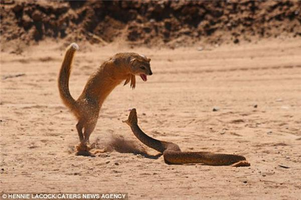
Sometimes, motion is the only cue 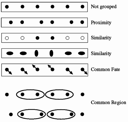 |
 |
motion and perceptual organization
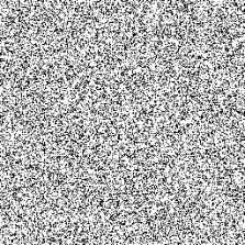

motion and perceptual organization
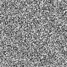
motion and perceptual organization
Even "impoverished" motion data can evoke a strong precept

motion and perceptual organization
motion and perceptual organization
Experimental study of apparent behavior. Fritz Heider & Marianne Simmel. 1944
“With Fritz Heider, Simmel co-authored 'An Experimental Study of Apparent Behavior,' which explored the experience of animacy. The study showed that subjects presented with a certain display of inanimate two-dimensional figures are inclined to ascribe intentions to those figures. This result has been taken to establish "the human instinct for storytelling" and to serve as important data in the study of theory of mind.
”
motion and perceptual organization
more applications of motion
- Segmentation of objects in space and time
- Estimating 3D structure
- Learning dynamical models—how things move
- Recognizing events and activities
- Improving video quality (motion stabilization)
motion estimation techniques
Feature-based methods
- Extract visual features (corners, textured areas) and track them over multiple frames
- Sparse motion fields, but more robust tracking
- Suitable when image motion is large (10s of pixels)
Direct, dense methods
- Directly recover image motion at each pixel from spatio-temporal image brightness variations
- Dense motion fields, but sensitive to appearance variations
- Suitable for video and when image motion is small
motion estimation: optic flow
Optic flow is the apparent motion of objects or surfaces

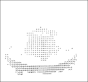
Will start by estimating motion of each pixel separately, then will consider motion of entire image
optical flow problem definition
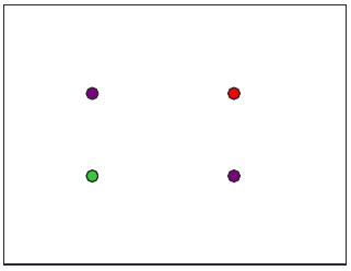
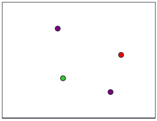
How to estimate pixel motion from image \(I(x,y,t)\) to \(I(x,y,t+1)\)?
optical flow problem definition
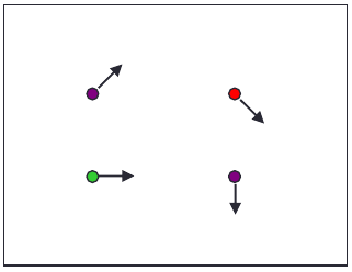

How to estimate pixel motion from image \(I(x,y,t)\) to \(I(x,y,t+1)\)?
- Solve pixel correspondence problem
- Given a pixel in \(I(x,y,t)\), look for nearby pixels of the same color in \(I(x,y,t+1)\)
optical flow problem definition


Key assumptions
- Color Constancy: a point in \(I(x,y,t)\) looks the same in \(I(x,y,t+1)\)
- for grayscale images, this is brightness constancy
- Small Motion: points do not move very far
This is called the optical flow problem
optical flow constraints (grayscale images)
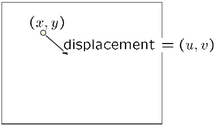
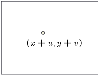
Let's look at these constraints more closely
- Brightness Constancy Constraint (equation) \[I(x,y,t) = I(x+u,y+v,t+1)\]
optical flow constraints (grayscale images)


Let's look at these constraints more closely
- Small Motion: (\(u\) and \(v\) are less than 1 pixel, or smooth)
Taylor series expansion of \(I\): \[I(x+u,y+v) = I(x,y) + \frac{\partial I}{\partial x} u + \frac{\partial I}{\partial y} v + [\text{higher order terms}]\] \[\approx I(x,y) + \frac{\partial I}{\partial x} u + \frac{\partial I}{\partial y} v\]
optical flow equation
Combining these two equations
\[\begin{array}{rcl} 0 & = & I(x+u,y+v,t+1) - I(x,y,t) \\ & \approx & I(x,y,t+1) + I_xu + I_yv - I(x,y,t) \end{array}\]
(short hand: \(I_x = \frac{\partial I}{\partial x}\) for \(t\) or \(t+1\))
optical flow equation
Combining these two equations
\[\begin{array}{rcl} 0 & = & I(x+u,y+v,t+1) - I(x,y,t) \\ & \approx & I(x,y,t+1) + I_xu + I_yv - I(x,y,t) \\ & \approx & \left[I(x,y,t+1) - I(x,y,t)\right] + I_xu + I_yv \\ & \approx & I_t + I_xu + I_yv \\ & \approx & I_t + \nabla I \cdot \left< u,v \right> \end{array}\]
In the limit as \(u\) and \(v\) go to zero, this becomes exact
\[0 = I_t + \nabla I \cdot \left< u,v \right>\]
Brightness constancy constraint equation
\[I_x u + I_y v + I_t = 0\]
how does this make sense?
Brightness constancy constraint equation
\[I_x u + I_y v + I_t = 0\]
What do the static image gradients have to do with motion estimation?

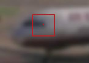
the brightness constancy constraint
Can we use this equation to recover image motion (\(u\), \(v\)) at each pixel?
\[0 = I_t + \nabla I \cdot \left< u,v \right> \quad\text{or}\quad I_xu + I_yv + I_t = 0\]
How many equations and unknowns per pixel?
- One equation (this is a scalar equation!), two unknowns (\(u\), \(v\))
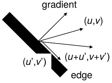
The component of the motion perpendicular to the gradient (i.e., parallel to the edge) cannot be measured
|
If \((u,v)\) satisfies the equation, so does \((u+u', v+v')\) if \(\nabla I \cdot [u'\,v']^T = 0\) |
 |
aperture problem

aperture problem
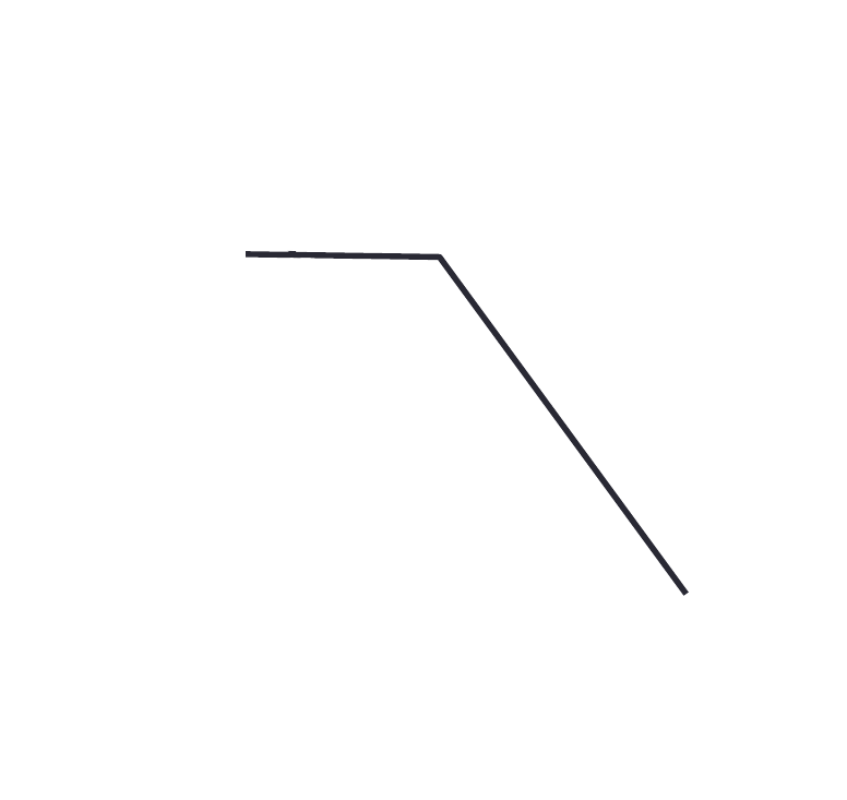
aperture problem

aperture problem

aperture problem

the barberpole illusion

the barberpole illusion

the barberpole illusion

solving the ambiguity
B.Lucas and T.Kanade. An iterative image registration technique with an application to stereo vision. In Proceedings of the International Joint Conference on Artificial Intelligence. pp. 674–679. 1981.
- How to get more equations for a pixel?
- Spatial coherence constraint
- Assume the pixel's neighbors have the same \((u,v)\)
- If we use a 5x5 window, that gives us 25 equations per pixel
\[0 = I_t(p_i) + \nabla I(p_i) \cdot [u\,v]\]
solving the ambiguity
Least squares problem! (\(A x = b\), where \(A\): 25x2, \(x\): 2x1, \(b\): 25x1)
\[\left[\begin{array}{cc} I_x(p_1) & I_y(p_1) \\ I_x(p_2) & i_y(p_2) \\ \vdots & \vdots \\ I_x(p_{25}) & I_y(p_{25}) \end{array}\right] \left[\begin{array}{c} u \\ v \end{array}\right] = -\left[\begin{array}{c} I_t(p_1) \\ I_t(p_2) \\ \vdots \\ I_t(p_{25}) \end{array}\right]\]
Overconstrained linear system
Least squares solution for \(x\) given by \((A^T A) x = A^T b\)
\[\left[\begin{array}{cc} \sum I_xI_x & \sum I_xI_y \\ \sum I_x I_y & \sum I_y I_y \end{array}\right] \left[\begin{array}{c} u \\ v \end{array}\right] = -\left[\begin{array}{c} \sum I_xI_t \\ \sum I_yI_t \end{array}\right]\]
The summations are over all pixels in the K\(\times\)K window
conditions for solvability
Optimal \((u,v)\) satisfies Lucas-Kanade equation
\[\left[\begin{array}{cc} \sum I_xI_x & \sum I_xI_y \\ \sum I_x I_y & \sum I_y I_y \end{array}\right] \left[\begin{array}{c} u \\ v \end{array}\right] = -\left[\begin{array}{c} \sum I_xI_t \\ \sum I_yI_t \end{array}\right]\]
When is this solvable? i.e., what are good points to track?
- \(A^TA\) should be invertible
- \(A^TA\) should not be too small due to noise
- eigenvalues \(\lambda_1\) and \(\lambda_2\) of \(A^TA\) should not be too small
- \(A^TA\) should be well-conditioned
- \(\lambda_1 / \lambda_2\) should not be too large (\(\lambda_1\) is larger eigenvalue)
Does this remind you of anything? (criteria of Harris corner detector)
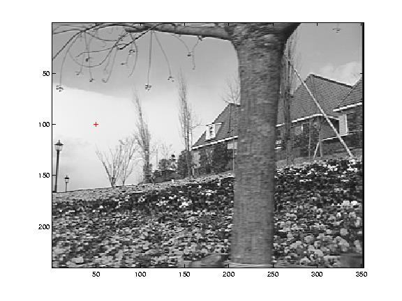
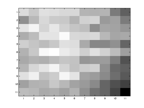
low texture region
 |
 |
\(\sum \nabla I(\nabla I)^T\)
- gradients have small magnitude
- small \(\lambda_1\), small \(\lambda_2\)
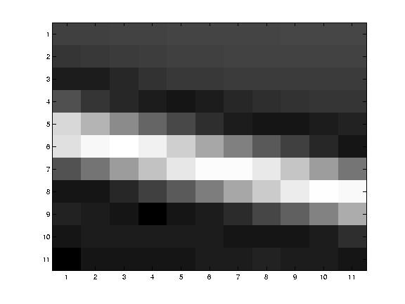
edge
 |
 |
\(\sum \nabla I(\nabla I)^T\)
- large gradients, all the same
- large \(\lambda_1\), small \(\lambda_2\)
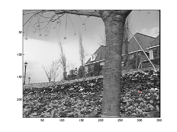
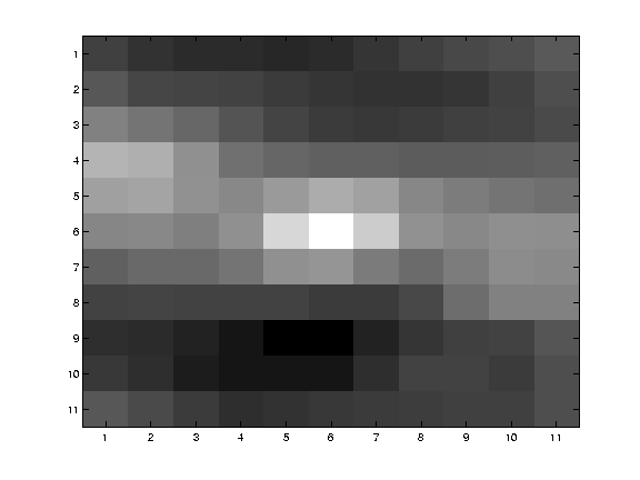
high textured region
 |
 |
\(\sum \nabla I(\nabla I)^T\)
- gradients are different, large magnitudes
- large \(\lambda_1\), large \(\lambda_2\)
the aperture problems solved

the aperture problems solved

the aperture problems solved

the aperture problems solved

errors in lucas-kanade
- A point does not move like its neighbors
- Motion segmentation
- Brightness constancy does not hold
- Do exhaustive neighborhood search with normalized correlation, tracking features, maybe SIFT, more later...
- The motion is large (larger than a pixel)
- Not-linear: iterative refinement
- Local minima: coarse-to-fine estimation
revisiting the small motion assumption

- Is this motion small enough?
- Probably not—it's much larger than one pixel
- How might we solve this problem?
optical flow: aliasing
Temporal aliasing causes ambiguities in optical flow because images can have many pixels with the same intensity. i.e., how do we know which "correspondence" is correct?
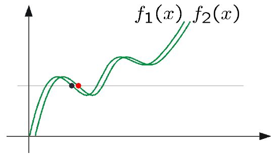

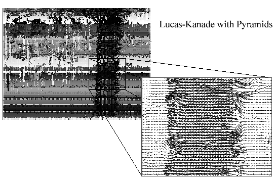
To overcome aliasing: coarse-to-fine estimation
reduce the resolution!

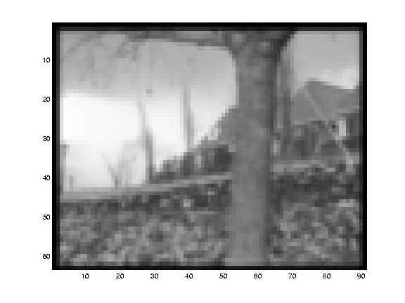


coarse-to-fine optical flow estimation
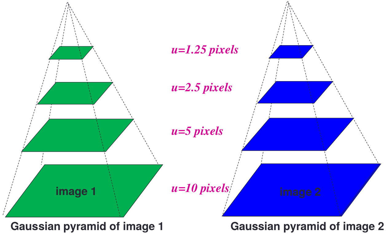
coarse-to-fine optical flow estimation

optical flow results
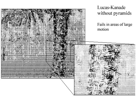
optical flow results
temporal aliasing in real life
state-of-the-art optical flow
Start with something similar to Lucas-Kanade
\(+\) gradient constancy
\(+\) energy minimization with smoothing term
\(+\) region matching
\(+\) keypoint matching (long-range)

optical flow
- Definition: optical flow is the apparent motion of brightness patterns in the image
- Ideally, optical flow would be the same as the motion field
- Have to be careful: apparent motion can be caused by lighting changes without any actual motion
- Think of a uniform rotating sphere under a fixed lighting vs. a stationary sphere under moving illumination
