Fitting and Alignment
COS 351 - Computer Vision
assign02
Any questions?
review: definitions
- Fitting
- find the parameters of a model that best fit the data
- Alignment
- find the parameters of the transformation that best align matched points
review: fitting and alignment
Design challenges
- Design a suitable goodness of fit measure
- Similarity should reflect application goals
- Encode robustness to outliers and noise
- Design an optimization method
- Avoid local optima
- Find best parameters quickly
fitting and alignment: methods
- Global optimization / Search for parameters
- Least squares fit
- Robust least squares
- Iterative Closest Point (ICP)
- Hypothesize and test
- Generalized Hough transform
- RANSAC
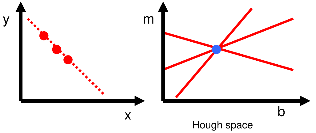
review: hough transform
- Create a grid of parameter values
- Each point votes for a set of parameters, incrementing those values in grid
- Find maximum or local maxima in grid
review: hough transform
P.V.C. Hough, Machine Analysis of Bubble Chamber Pictures, Proc. Int. Conf. High Energy Accelerators and Instrumentation, 1959.
Given a set of points, find the curve or line that explains the data points best
review: hough transform

Hough Transform
How would we find circles?
- of fixed radius
- of unknown radius
- of unknown radius but with known edge orientation
hough transform for circles
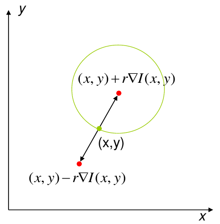
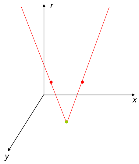
hough transform for circles
Conceptually equivalent procedure: for each \((x,y,r)\), draw the corresponding circle in the image and compute its "support"
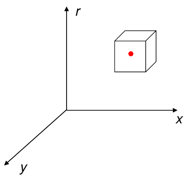
Is this more or less efficient than voting with features?
hough transform conclusions
Good
- Robust to outliers: each point votes separately
- Fairly efficient (much faster than trying all sets of parameters)
- Provides multiple good fits
Bad
- Some sensitivity to noise
- Bin size trades off between noise tolerance, precision, and speed/memory
- can be hard to find sweet spot
- Not suitable for more than a few parameters
- grid size grows exponentially
hough transform conclusions
Common applications
- Line fitting (also circles, ellipses, etc.)
- Object instance recognition (parameters are affine transform)
- Object category recognition (parameters are position/scale)
RANSAC
RANdom SAmple Consensus (RANSAC)
- Sample (randomly) the number of points required to fit the model
- Solve for model parameters using samples
- Score by the fraction of inliers within a preset threshold of the model
- Repeat 1–3 until the best model is found with high confidence
RANSAC
Line fitting example
RANSAC
Line fitting example
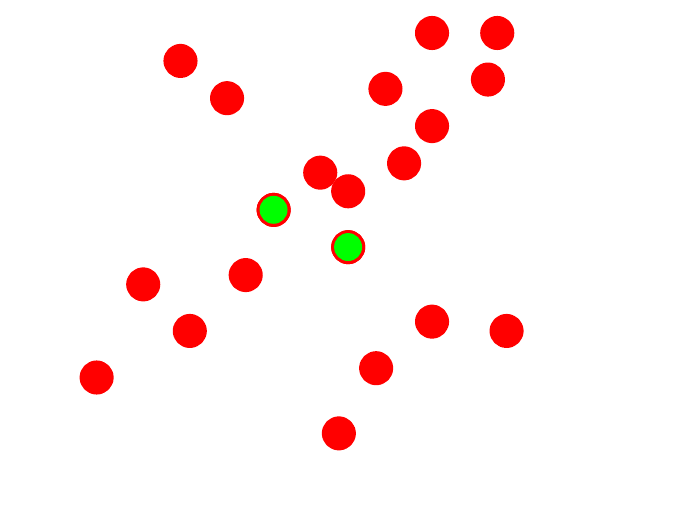
RANSAC
Line fitting example
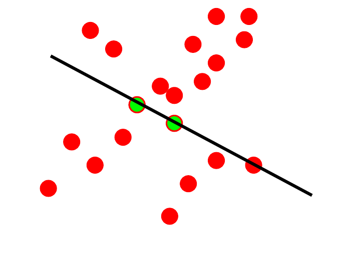
RANSAC
Line fitting example

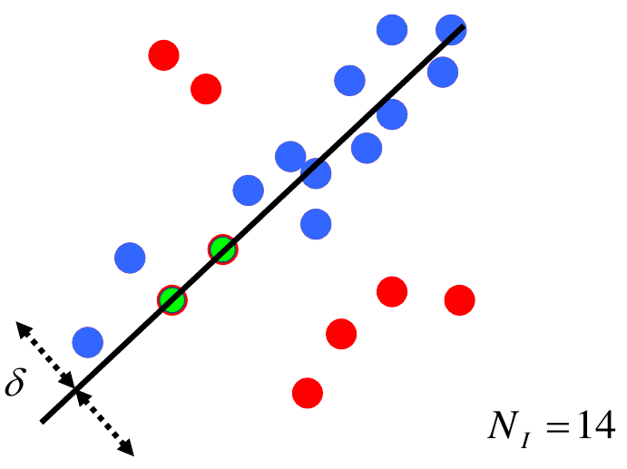
RANSAC
Line fitting example
how to choose parameters?
- Number of samples \(N\)
- choose \(N\) so that, with probability \(p\), at least one random sample is free from outliers (e.g., \(p=0.99\)) (outlier ratio: \(e\))
- Number of sampled points \(s\)
- minimum number needed to fit the model
- Distance threshold \(\delta\)
- Choose \(\delta\) so that a good point with noise is likely (e.g., \(\textrm{prob}=0.95\)) within threshold
- zero-mean Gaussian noise with std.dev \(\sigma\): \(t^2 = 3.84 \sigma^2\)
\[N = \frac{\log(1-p)}{\log(1-(1-e)^s)}\]
how to choose parameters?
\[N = \frac{\log(1-p)}{\log(1-(1-e)^s)}\]
Proportion of outliers \(e\) for \(p = 0.99\)
| s | 5% | 10% | 20% | 25% | 30% | 40% | 50% |
|---|---|---|---|---|---|---|---|
| 2 | 2 | 3 | 5 | 6 | 7 | 11 | 17 |
| 3 | 3 | 4 | 7 | 9 | 11 | 19 | 35 |
| 4 | 3 | 5 | 9 | 13 | 17 | 34 | 72 |
| 5 | 4 | 6 | 12 | 17 | 26 | 57 | 146 |
| 6 | 4 | 7 | 16 | 24 | 37 | 97 | 293 |
| 7 | 4 | 8 | 20 | 33 | 54 | 163 | 588 |
| 8 | 5 | 9 | 26 | 44 | 78 | 272 | 1177 |
ransac conclusions
Good
- Robust to outliers
- Applicable for larger number of objective function parameters than Hough transform
- Optimization parameters are easier to choose than Hough transform
Bad
- Computational time grows quickly with fraction of outliers and number of parameters
- Not good for getting multiple fits
ransac conclusions
Common applications
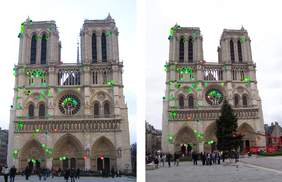
- Computing a homography (e.g., image stitching)
- Estimating fundamental matrix (relating two views)
how do we fit the best alignment?
alignment
- Alignment
- find parameters of model that maps one set of points to another
Typically want to solve for a global transformation that accounts for most true correspondences
Difficulties
- Noise (typically 1–3 pixels)
- Outliers (often 50%)
- Many-to-one matches or multiple objects
parametric (global) warping
Transformation \(T\) is a coordinate-changing machine:
\[\mathbf{p}' = T(\mathbf{p})\]
What does it mean that \(T\) is global?
- is the same for any point \(p\)
- can be described by just a few numbers (parameters)
parametric (global) warping
For linear transformations, we can represent \(T\) as a matrix
\[\mathbf{p}' = \mathbf{T}(\mathbf{p})\]
\[\left[\begin{array}{c} x' \\ y' \end{array}\right] = \mathbf{T}\ \left[\begin{array}{c} x \\ y \end{array}\right]\]
common transformations
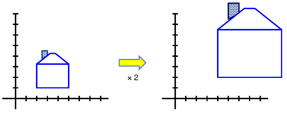
scaling
Scaling a coordinate means multiplying each of its components by a scalar
Uniform scaling means this scalar is the same for all components
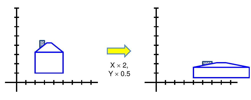
scaling
Scaling a coordinate means multiplying each of its components by a scalar
Non-uniform scaling means different scalars per component
scaling
Scaling operation
\[x' = ax,\quad y' = by\]
or in matrix form
\[\left[\begin{array}{c} x' \\ y' \end{array}\right] = \mathbf{S}\ \left[\begin{array}{c} x \\ y \end{array}\right] = \left[\begin{array}{cc} a & 0 \\ 0 & b \end{array}\right] \left[\begin{array}{c} x \\ y \end{array}\right]\]
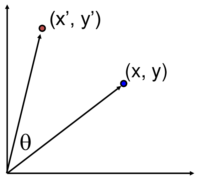
2D rotation
\[x' = x \cos(\theta) - y \sin(\theta)\] \[y' = x \sin(\theta) - y \cos(\theta)\]
2D rotation
This is easy to capture in matrix form:
\[\left[\begin{array}{c} x' \\ y' \end{array}\right] = \mathbf{R}\ \left[\begin{array}{c} x \\ y \end{array}\right] = \left[\begin{array}{cc} \cos(\theta) & -\sin(\theta) \\ \sin(\theta) & \cos(\theta) \end{array}\right] \left[\begin{array}{c} x \\ y \end{array}\right]\]
Even though \(\sin(\theta)\) and \(\cos(\theta)\) are nonlinear functions of \(\theta\),
- \(x'\) is a linear combination of \(x\) and \(y\)
- \(y'\) is a linear combination of \(x\) and \(y\)
What is the inverse transformation?
- Rotation by \(-\theta\)
- For rotation matrices: \(\mathbf{R}^{-1} = \mathbf{R}^T\)
basic 2d transformations
|
Scale: \[\left[\begin{array}{c} x' \\ y' \end{array}\right] = \left[\begin{array}{cc} s_x & 0 \\ 0 & s_y \end{array}\right] \left[\begin{array}{c} x \\ y \end{array}\right]\] Shear: \[\left[\begin{array}{c} x' \\ y' \end{array}\right] = \left[\begin{array}{cc} 1 & \alpha_x \\ \alpha_y & 1 \end{array}\right] \left[\begin{array}{c} x \\ y \end{array}\right]\] |
Rotate: \[\left[\begin{array}{c} x' \\ y' \end{array}\right] = \left[\begin{array}{cc} \cos(\theta) & -\sin(\theta) \\ \sin(\theta) & \cos(\theta) \end{array}\right] \left[\begin{array}{c} x \\ y \end{array}\right]\] Translate: \[\left[\begin{array}{c} x' \\ y' \end{array}\right] = \left[\begin{array}{ccc} 1 & 0 & t_x \\ 0 & 1 & t_y \end{array}\right] \left[\begin{array}{c} x \\ y \\ 1 \end{array}\right]\] |
basic 2d transformations
Affine is any combination of:
- Linear transformations (scale, rotation, shear), and
- Translations
\[\left[\begin{array}{c} x' \\ y' \end{array}\right] = \left[\begin{array}{ccc} a & b & c \\ d & e & f \end{array}\right] \left[\begin{array}{c} x \\ y \\ 1 \end{array}\right], \textrm{ or } \left[\begin{array}{c} x' \\ y' \\ 1 \end{array}\right] = \left[\begin{array}{ccc} a & b & c \\ d & e & f \\ 0 & 0 & 1 \end{array}\right] \left[\begin{array}{c} x \\ y \\ 1 \end{array}\right]\]
Properties of affine transformations:
- Lines map to lines
- Parallel lines remain parallel
- Ratios are preserved
- Closed under composition
projective transformations
Projective transformations are combinations of:
- Affine transformations, and
- Projective warps
\[\left[\begin{array}{c} x' \\ y' \\ w' \end{array}\right] = \left[\begin{array}{ccc} a & b & c \\ d & e & f \\ g & h & i \end{array}\right] \left[\begin{array}{c} x \\ y \\ w \end{array}\right]\]
Properties of projective transformations:
|
|
2d image transformations (ref table)
example: solving for translation
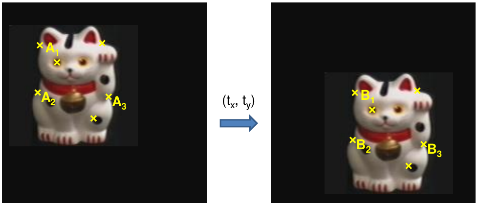
Given matched points in \(\{A\}\) and \(\{B\}\), estimate the translation of the object
\[\left[\begin{array}{c} x_i^B \\ y_i^B \end{array}\right] = \left[\begin{array}{c} x_i^A \\ y_i^A \end{array}\right] + \left[\begin{array}{c} t_x \\ t_y \end{array}\right]\]
example: solving for translation
Least squares solution
|
\[\left[\begin{array}{c} x_i^B \\ y_i^B \end{array}\right] = \left[\begin{array}{c} x_i^A \\ y_i^A \end{array}\right] + \left[\begin{array}{c} t_x \\ t_y \end{array}\right]\] \[\left[\begin{array}{cc} 1 & 0 \\ 0 & 1 \\ \vdots & \vdots \\ 1 & 0 \\ 0 & 1 \end{array}\right] \left[\begin{array}{c} t_x \\ t_y \end{array}\right] = \left[\begin{array}{c} x_1^B - x_1^A \\ y_1^B - y_1^A \\ \vdots \\ x_n^B - x_n^A \\ y_n^B - y_n^A \end{array}\right]\] |
example: solving for translation
RANSAC solution
- Sample a set of matching points (1 pair)
- Solve for transformation parameters
- Score parameters with number of inliers
- Repeat steps 1–3 \(N\) times
\[\left[\begin{array}{c} x_i^B \\ y_i^B \end{array}\right] = \left[\begin{array}{c} x_i^A \\ y_i^A \end{array}\right] + \left[\begin{array}{c} t_x \\ t_y \end{array}\right]\]
example: solving for translation
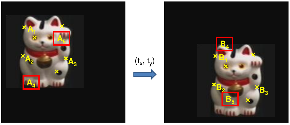
RANSAC solution problem: outliers
example: solving for translation
Hough transform solution
- Initialize a grid of parameter values
- Each matched pair casts a vote for consistent values
- Find the parameters with the most votes
- Solve using least squares with inliers
\[\left[\begin{array}{c} x_i^B \\ y_i^B \end{array}\right] = \left[\begin{array}{c} x_i^A \\ y_i^A \end{array}\right] + \left[\begin{array}{c} t_x \\ t_y \end{array}\right]\]
example: solving for translation
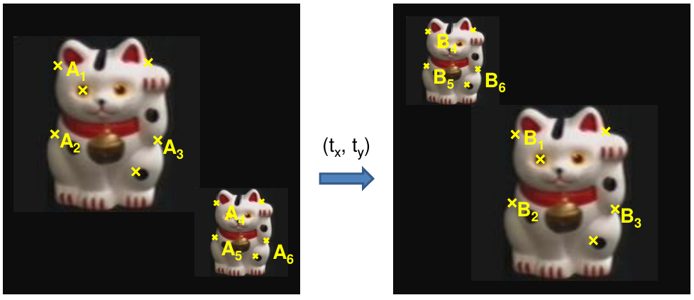
Hough transform solution problem: outliers, multiple objects, and/or many-to-one matches
example: solving for translation
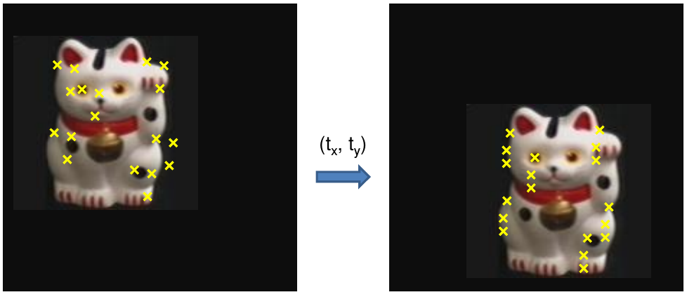
Problem: no initial guesses for correspondences
\[\left[\begin{array}{c} x_i^B \\ y_i^B \end{array}\right] = \left[\begin{array}{c} x_i^A \\ y_i^A \end{array}\right] + \left[\begin{array}{c} t_x \\ t_y \end{array}\right]\]
alignment without prior matched pairs
What if you want to align but have no prior matched pairs?
- Hough transform and RANSAC not applicable
- Important applications
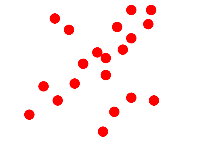
iterative closest points (ICP) algorithm
Goal: estimate transform between two dense sets of points
- Initialize transformation (e.g., compute differences in means and scales)
- Assign each point in \(\{A\}\) to its nearest neighbor in \(\{B\}\)
- Estimate transformation parameters
- e.g., least squares or robust least squares
- Transform the points in \(\{A\}\) using estimated parameters
- Repeat steps 2–4 until change is very small
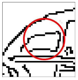
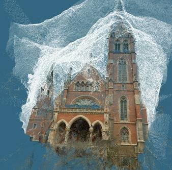
example: aligning boundaries
- Extract edge pixels \(p_1, \ldots, p_n\) and \(q_1, \ldots, q_m\)
- Compute initial transformation (e.g., compute translation and scaling by center of mass, variance within each image)
- Get nearest neighbors: for each point \(p_i\) find corresponding \(\textrm{match}(i) = \argmin{j} \textrm{dist}(p_i, q_j)\)
- Compute transformation \(\mathbf{T}\) based on matches
- Warp points \(\mathbf{p}\) according to \(\mathbf{T}\)
- Repeat 3–5 until convergence
example: aligning boundaries
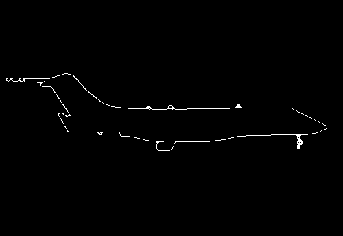
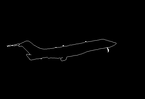
example: aligning boundaries
example: solving for translation
ICP solution
- Find nearest neighbors for each point
- Compute transform using matches
- Move points using transform
- Repeat steps 1–3 until convergence
example: solving for translation
Problem: no initial guesses for correspondences
\[\left[\begin{array}{c} x_i^B \\ y_i^B \end{array}\right] = \left[\begin{array}{c} x_i^A \\ y_i^A \end{array}\right] + \left[\begin{array}{c} t_x \\ t_y \end{array}\right]\]
Sparse ICP
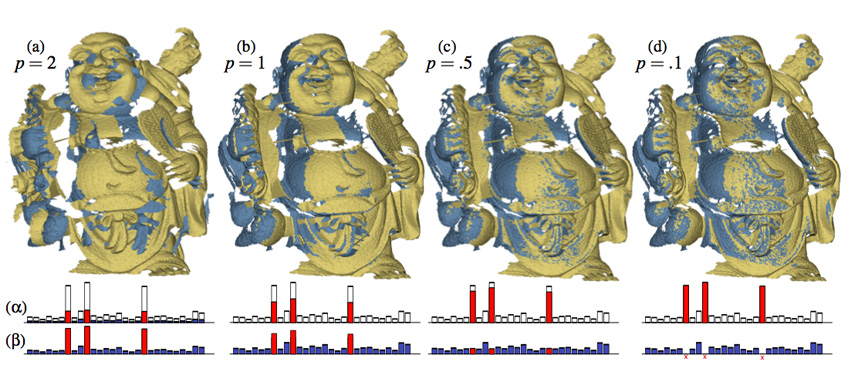
Sparse Iterative Closest Point. Sofien Bouaziz, Andrea Tagliasacchi, Mark Pauly. site
algorithm summaries
- Least Squares Fit
- closed form solution
- robust to noise
- not robust to outliers
- Robust Least Squares
- improves robustness to noise
- requires iterative optimization
- Hough transform
- robust to noise and outliers
- can fit multiple models
- only works for a few parameters (1–4 typically)
algorithm summaries
- RANdom SAmpling Consensus (RANSAC)
- robust to noise and outliers
- works with a moderate number of parameters (e.g., 1–8)
- Iterative Closest Point (ICP)
- For local alignment only; does not require initial correspondences