Templates, Image Pyramids, Filter Banks

COS 351 - Computer Vision

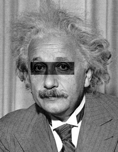
template matching

Goal: find in image Main challenge: What is a good similarity or distance measure between two patches? Correlation Zero-mean correlation Sum Square Difference Normalized Cross Correlation

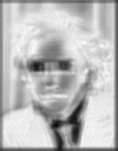
matching with filters

Goal: find in image

Method 0: filter the image with eye patch

\[h[m,n] = \sum_{k,l} g[k,l] f[m+k,n+l]\]

\(f\) is image, \(g\) is filter

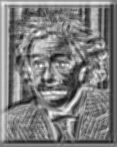
matching with filters

Goal: find in image

Method 1: filter the image with zero-mean eye

\[h[m,n] = \sum_{k,l} (g[k,l])-\overline{g}) f[m+k,n+l]\]

\(\overline{g}\) is mean of \(g\)

matching with filters

Goal: find in image

Method 2: SSD

\[h[m,n] = \sum_{k,l} (g[k,l])-f[m+k,n+l])^2\]

\(\overline{f}\) is mean of \(f\)

matching with filters

Goal: find in image

Method 2: SSD

\[h[m,n] = \sum_{k,l} (g[k,l])-f[m+k,n+l])^2\]

What is the potential downside?

matching with filters

Goal: find in image

Method 3: Normalized cross-correlation

\[h[m,n] = \frac{\sum_{k,l} (g[k,l])-\overline{g})(f[m-k,n-l]-\overline{f}_{m,n})}{\left( \sum_{k,l}(g[k,l] - \overline{g})^2 \sum_{k,l}(f[m-k,n-l]-\overline{f}_{m,n})^2 \right)^{0.5}}\]

MATLAB: normxcorr2(template, im)

matching with filters

Goal: find in image

Method 3: Normalized cross-correlation

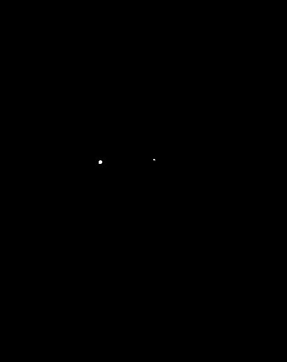
matching with filters

Goal: find in image

Method 3: Normalized cross-correlation

q: what is the best method to use?

a. depends

• SSD: faster, sensitive to overall intensity
• Normalized cross-correlation: slower, invariant to local average intensity and contrast
• But really, neither of these baselines are representative of modern recognition

q: what if we want to find larger or smaller eyes?

a. Use image pyramid to find

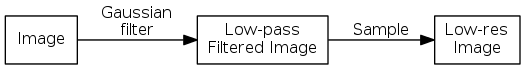
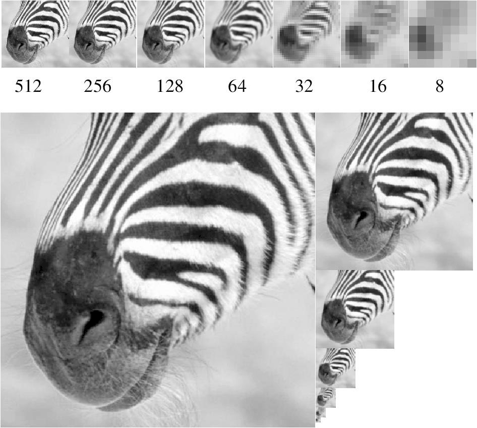
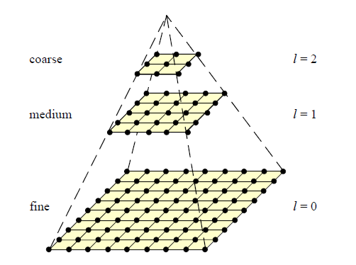
review of sampling

gaussian pyramid

template matching with image pyramids

input: image, template

1. match template at current scale
2. downsample image
3. repeat steps 1 and 2 until image is very small
4. take responses above some threshold, perhaps with non-maxima suppression

2d edge detection filters

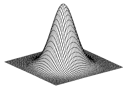
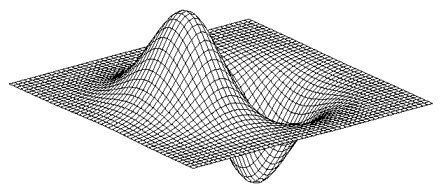
\[h_\sigma(u,v) = \frac{1}{2 \pi \sigma^2} e^{-\frac{u^2+v^2}{2 \sigma^2}},\quad \frac{\partial}{\partial x} h_\sigma(u,v),\quad \nabla^2 h_\sigma(u,v)\]

\(\nabla^2\) is the Laplacian operator:

\[\nabla^2 f = \frac{\partial^2 f}{\partial x^2} + \frac{\partial^2 f}{\partial y^2}\]

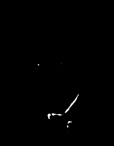
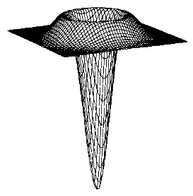
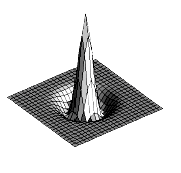
laplacian filter

\(-\) \(\approx\)

computing gaussian/laplacian pyramid

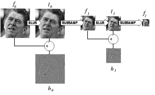
Can we reconstruct the original from the Laplacian pyramid?

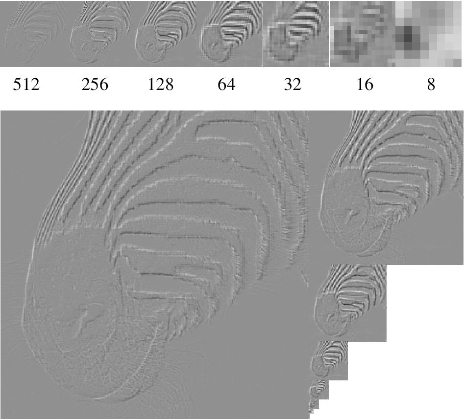
laplacian pyramid

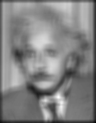
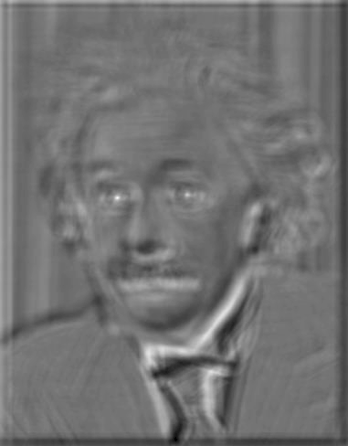
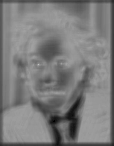
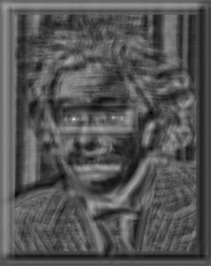
hybrid image

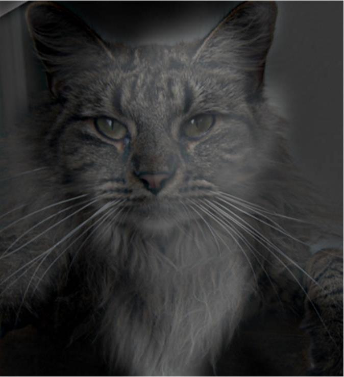
hybrid image in laplacian pyramid

high frequency -> low frequency

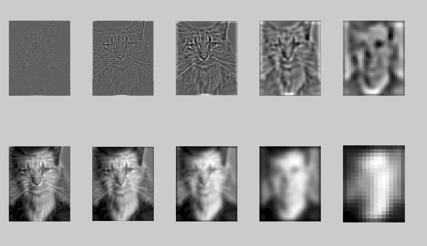
image representation

• Pixels

  • great for spatial resolution
  • poor access to frequency

• Fourier transform

  • great for frequency
  • not for spatial info

• Pyramid/filter banks

  • balance between spatial and frequency information

major uses of image pyramids

• compression
• object detection
  • scale search
  • features
• detecting stable interest points
• registration
  • coarse-to-fine

coarse-to-fine image registration

1. Compute Gaussian pyramid
2. Align with coarse pyramid
3. Successively align with finer pyramids
   • Search smaller range

Why is this faster?

Are we guaranteed to get the same result?

compression

How is it that a 4MP image can be compressed to a few hundred KB without a noticeable change?

4MP = 4 million pixels = 2000 pixels x 2000 pixels

If storing 8bits/channel (RGB), each pixel uses 24bits = 3bytes.

\[4\text{MP} * 3\text{B/P} = 12,000,000\text{B} \approx 11,718\text{KB} \approx 11.5\text{MB} \]

lossy image compression (JPEG)

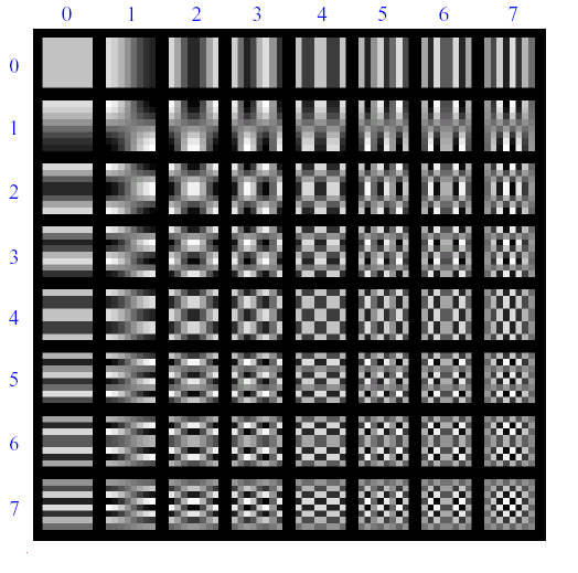
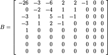
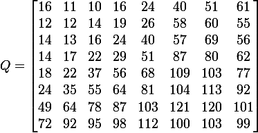
Block-based Discrete Cosine Transform (DCT)

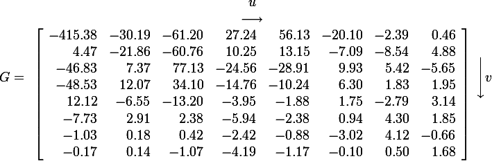
using dct in jpeg

• The first coefficient B(0,0) is the DC component, the average intensity
• The top-left coeffs represent low frequencies, the bottom-right high frequencies.

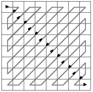
image compression using DCT

• Quantize
  • More coarsely for high frequencies (which also tend to have smaller values)
  • Many quantized high frequency values will be zero
• Encode
  • Can decode with inverse DCT

jpeg compression summary

1. Convert image to YCrCb
2. Subsample color by factor of 2
   • People have bad resolution for color
3. Split into blocks (8x8, typically), subtract 128
4. For each block
   1. Compute DCT coefficients
   2. Coarsely quantize
      • Many high frequency components will become zero
   3. Encode (e.g., with Huffman coding)

reconstruction

“

Left: a final image is built up from a series of basis functions. Right: each of the DCT basis functions that comprise the image, and the corresponding weighting coefficient. Middle: the basis function, after multiplication by the coefficient: this component is added to the final image. For clarity, the 8x8 macroblock in this example is magnified by 10x using bilinear interpolation.

”