Thinking in Frequency
COS 351 - Computer Vision
recap
- Linear filtering is dot product at each position
- not a matrix multiplication
- can smooth, sharpen, translate (among many other uses)
- Be aware of details for filter size, extrapolation, cropping
thinking in frequency
- Fourier transform and frequency domain
- frequency view of filtering
- hybrid images
- sampling
- Reminder: Read your textbook!
- This lecture covers material in 3.4
Gaussian
Why does the Gaussian give a nice smooth image, but the square filter give edgy artifacts?


hybrid images

hybrid images
Why do we get different, distance-dependent interpretations of hybrid images?


subsampling
Why does a lower resolution image still make sense to us? What do we lose?


Thinking in terms of frequency
Jean Baptiste Joseph Fourier (1768–1830)
Fourier had crazy idea in 1807:
“Any univariate function can be rewritten as a weighted sum of sines and cosines of different frequencies
”

Jean Baptiste Joseph Fourier (1768–1830)
Don't believe it?
- Neither did Lagrange, Laplace, Poisson, and other big wigs
- Not translated into English until 1878!


Jean Baptiste Joseph Fourier (1768–1830)
But it's (mostly) true!
- called Fourier Series
- there are some subtle restrictions
“... the manner in which the author arrives at these equations is not exempt of difficulties and ... his analysis to integrate them still leaves something to be desired on the score of generality and even rigour.
”
Jean Baptiste Joseph Fourier (1768–1830)
French mathematician who discovered that any periodic motion can be written as a superposition of sinusoidal and cosinusoidal vibrations. He developed a mathematical theory of heat in Theorie Analytique de la Chaleur (Analytic Theory of Heat) (1822), discussing it in terms of differential equations.
Fourier was a friend and advisor of Napolean. Fourier believed that his health would be improved by wrapping himself up in blankets, and in this state he tripped down the stairs in his house and killed himself. The paper of Galois which he had taken home to read shortly before his death was never recovered.
How would math have changed if the Slanket or Snuggie had been invented?
Jean Baptiste Joseph Fourier (1768–1830)

a sum of sines
|
Our building block: \[ A \sin(\omega x + \phi) \] Add enough of them to get any signal \(g(x)\) you want! |
 |
frequency spectra
example: \(g(t) = sin(2 \pi f t) + (1/3) \sin(2 \pi(3f) t)\)
 \(=\)
\(=\)
 \(+\)
\(+\)


frequency spectra
How do we create this wave?

frequency spectra
How do we create this wave?

 \(+\)
\(+\)
 \(=\)
\(=\)

frequency spectra
How do we create this wave?

 \(+\)
\(+\)
 \(=\)
\(=\)

frequency spectra
How do we create this wave?

 \(+\)
\(+\)
 \(=\)
\(=\)

frequency spectra
How do we create this wave?

 \(+\)
\(+\)
 \(=\)
\(=\)

frequency spectra
How do we create this wave?

 \(+\)
\(+\)
 \(=\)
\(=\)

frequency spectra
How do we create this wave?

\[= A \sum_{k=1}^\infty \frac{1}{k} \sin(2 \pi kt)\]

example: music
We think of music in terms of frequencies at different magnitudes

other signals
We can also think of all kinds of other signals the same way

fourier analysis in images
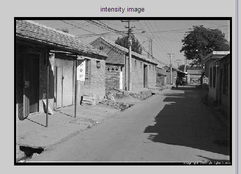
Intensity Image:


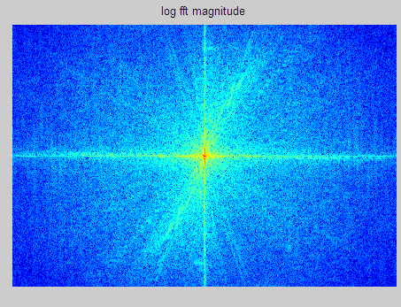
Fourier Image:


fourier transform
Fourier transform stores the magnitude and phase at each frequency
- Magnitude encodes how much signal there is at a particular frequency
- Phase encodes spatial information (indirectly)
- For mathematical convenience, this is often notated in terms of real and complex numbers
Amplitude: \(A = \pm \sqrt{R(\omega)^2 + I(\omega)^2}\)
Phase: \(\phi = \tan^{-1} \frac{I(\omega)}{R(\omega)}\)
Salvador Dali invented Hybrid images?

Salvador Dali invented Hybrid images?

Salvador Dali invented Hybrid images?

fourier bases
Teases away fast vs. slow changes in the image

This change of basis is the Fourier Transform
In MATLAB, check out: imagesc(log(abs(ffshift(fft2(im)))));
man-made scene


can change spectrum, then reconstruct

low and high pass filtering


the convolution theorem
The Fourier transform of the convolution of two functions is the product of their Fourier transforms
\[F[g * h] = F[g] F[h]\]
Convolution in spatial domain is equivalent to multiplication in frequency domain!
\[g*h = F^{-1}[F[g] F[h]]\]
filtering in spatial domain
| 1 | 0 | -1 |
| 2 | 0 | -2 |
| 1 | 0 | -1 |
 \(*\)
\(*\)
 \(=\)
\(=\)

filtering in frequency domain
FFT on image and kernel
 \(\Rightarrow\)

 \(\Rightarrow\)

filtering in frequency domain
Multiply FFT of image and FFT of kernel
 \(\times\)
 \(=\)
\(=\)

filtering in frequency domain
Inverse FFT of result
 \(\Rightarrow\)

FFT in matlab
Filtering with FFT
im = double(imread('...'))/255;
im = rgb2gray(im); % im should be a gray-scale floating point image
[imh,imw] = size(im);

hs = 50; % filter half-size
fil = fspecial('gaussian', hs*2+1, 10);

fftsize = 1024; % should be order of 2 (for speed) and incl. padding
im_fft  = fft2(im, fftsize, fftsize);  % 1) fft im with padding
fil_fft = fft2(fil, fftsize, fftsize); % 2) fft fil, pad to same
                                       %    size as im
im_fil_fft = im_fft .* fil_fft;        % 3) multiply fft images
im_fil = ifft2(im_fil_fft);            % 4) inverse fft2
im_fil = im_fil(1+hs:imh+hs, 1+hs:imw+hs); % 5) remove padding
Displaying with fft
figure(1), imagesc(log(abs(fftshift(im_fft)))), axis image, colormap jet
filtering
Why does the Gaussian give a nice smooth image, but the square filter give edgy artifacts?


Gaussian

box filter

sampling
Why does a lower resolution image still make sense to us? What do we lose?


subsampling by a factor of 2
Throw away every other row and column to create a 1/2 size image


aliasing problem
1D example (sine wave)

aliasing problem
1D example (sine wave)

aliasing problem
- Sub-sampling may be dangerous...
- Characteristic errors may appear:
- "Wagon wheels rolling the wrong way in movies"
- "Checkerboards disintegrate in ray tracing"
- "Striped shirts look funny on color television"
aliasing in video
Imagine a spoked wheel moving to the right (rotating clockwise). Mark wheel with dot so we can see what's happening.
If camera shutter is only open for a fraction of a frame tme (frame time = 1/30 sec for video, 1/24 sec for film):

Without dot, wheel appears to be rotating slowly backwards! (counterclockwise)
aliasing in graphics

sampling and aliasing

nyquist-shannon sampling theorem
-
When sampling a signal at discrete intervals, the sampling frequency must be \(\geq 2 * f_{\max}\)
-
\(f_{\max}\) is max frequency of the input signal
-
This will allow to reconstruct the original perfectly from the sampled version

anti-aliasing
Solutions:
-
Sample more often
-
Get rid of all frequencies that are greater than half the new sampling frequency
- will lose information
- but it's better than aliasing
- apply a smoothing filter
algorithm for downsampling by factor of 2
- Start with
image(h,w) -
Apply low-pass filter
im_blur = imfilter(image, fspecial('gaussian', 7, 1)) -
Sample every other pixel
im_small = im_blur(1:2:end, 1:2:end);
anti-aliasing

subsampling without pre-filtering


subsampling with gaussian pre-filtering


clues from human perception
- Early processing in humans filters for various orientations and scales of frequency
- Perceptual cues in the mid-high frequencies dominate perception
- When we see an image from far away, we are effectively subsampling it

campbell-robson contrast sensitivity curve

hybrid image in FFT
Hybrid image in FFT is low-pass image plus high-pass image
 \(=\)
\(=\)
 \(+\)
\(+\)

things to remember
|
 |
