using monte carlo integration
to solve the rendering equation

dr. jon denning
assistant professor of cse
taylor university

Frank S. Brenneman Lecture Series

the rendering equation

computer-generated photo-realistic images are created by accurately simulating the way light interacts with the world

good simulations require good modeling of lighting, materials, lenses, and the transport of light

the rendering equation

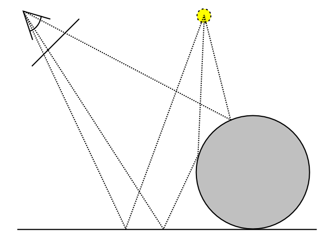
rendering systems, such as a ray tracer or path tracer, use the rendering equation to describe how the light bounces around the virtual scene until it enters the camera's lens

\[L_o (\mathbf{x}, \omega_o) = L_e(\mathbf{x}, \omega_o) + \int_\Omega \rho(\mathbf{x}, \omega_i, \omega_o) L_i(\mathbf{x}, \omega_i) (\omega_i \cdot \mathbf{n}) d\omega_i\]

the rendering equation describes the total amount of light (\(L_o\)) leaving from a point (\(\mathbf{x}\)) along a particular direction (\(\omega_o\)) given a function for all incoming light (\(L_i\)) about the hemisphere (\(\Omega\)) and a reflectance function (\(\rho\))

the rendering equation

\[L_o (\mathbf{x}, \omega_o) = L_e(\mathbf{x}, \omega_o) + \int_\Omega \rho(\mathbf{x}, \omega_i, \omega_o) L_i(\mathbf{x}, \omega_i) (\omega_i \cdot \mathbf{n}) d\omega_i\]

\(L_e\) and \(\rho\) are relatively easy to define well, and the equation is fairly straight-forward, yet the results from such a simple equation can be quite stunning

solving the rendering equation

so, how do we (efficiently) solve this?

\[L_o (\mathbf{x}, \omega_o) = L_e(\mathbf{x}, \omega_o) + \int_\Omega \rho(\mathbf{x}, \omega_i, \omega_o) L_i(\mathbf{x}, \omega_i) (\omega_i \cdot \mathbf{n}) d\omega_i\]

notes:

• \(\Omega\) is 2D domain (hemisphere)
• the equation is recursively defined (\(L_o\), \(L_i\))
• the function \(L_i\) is not well-behaved in general
  • discontinuous

solving the rendering equation

so, how do we (efficiently) solve this?

\[L_o (\mathbf{x}, \omega_o) = L_e(\mathbf{x}, \omega_o) + \int_\Omega \rho(\mathbf{x}, \omega_i, \omega_o) L_i(\mathbf{x}, \omega_i) (\omega_i \cdot \mathbf{n}) d\omega_i\]

monte carlo integration to the rescue!

note

in the interest of time, the focus of this talk is to provide intuition and motivation, not necessarily for a deeper understanding of the application of statistics or in computer graphics

just sit back and enjoy

integrals and averages

integral of a function over a domain

\[\int_{\mathbf{x}\in D} f(\mathbf{x}) dA_\mathbf{x}\]

"size" of a domain

\[A_D = \int_{\mathbf{x} \in D} dA_\mathbf{x}\]

average of a function over a domain

\[\frac{\int_{\mathbf{x}\in D} f(\mathbf{x}) dA_\mathbf{x}}{\int_{\mathbf{x} \in D} dA_\mathbf{x}} = \frac{\int_{\mathbf{x}\in D} f(\mathbf{x}) dA_\mathbf{x}}{A_D}\]

integrals and averages examples

average "daily" snowfall in Hillsboro last year

• domain: year, time interval (1D)
• integration variable: "day" of the year
• function: snowfall of "day"

\[\frac{\int_{\mathit{day}\in\mathit{year}} s(\mathit{day}) d\mathit{length}(\mathit{day})}{\mathit{length}(\mathit{year})}\]

integrals and averages examples

"today" average snowfall in Kansas

• domain: Kansas, surface (2D)
• integration variable: "location" in Kansas
• function: snowfall of "location"

\[\frac{\int_{\mathit{location}\in\mathit{Kansas}} s(\mathit{location})d\mathit{area}(\mathit{location})}{\mathit{area}(\mathit{location})}\]

integrals and averages examples

"average" snowfall in Kansas per day this year

• domain: Kansas \(\times\) year, area \(\times\) time (3D)
• integration variables: "location" and "day" in Kansas this year
• function: snowfall of "location" and "day"

\[\frac{\int_{\mathit{day}\in\mathit{year}}\int_{\mathit{loc}\in\mathit{KS}} s(\mathit{loc},\mathit{day}) d\mathit{area}(\mathit{loc})d\mathit{length}(\mathit{day})}{ \mathit{area}(\mathit{loc}) \mathit{length}(\mathit{day})}\]

discrete random variable

• random variable: \(x\)
• values: \(x_0\), \(x_1\), ..., \(x_n\)
• probabilities: \(p_0\), \(p_1\), ..., \(p_n\), where \(\sum_{j=1}^n p_j = 1\)
• example: rolling a die
  • values: \(x_1 = 1\), \(x_2 = 2\), \(x_3 = 3\), \(x_4 = 4\), \(x_5 = 5\), \(x_6 = 6\)
  • probabilities: \(p_1 = p_2 = p_3 = p_4 = p_5 = p_6 = \frac{1}{6}\)

expected value and variance

• expected value: \(E[x] = \sum_{j=1}^n v_jp_j\)
  • average value of the variable
• variance: \(\sigma^2[x] = E[(x - E[x])^2] = E[x^2] + E[x]^2\)
  • how much different from the average
• example: rolling a die
  • expected value: \(E[x] = (1+2+3+4+5+6)/6 = 3.5\)
  • variance: \(\sigma^2[x] =\, ... = 2.917\)

estimating expected values

• to estimate the expected value of a variable
  • choose a set of random values based on the probability
  • average their results

\[E[x] \approx \frac{1}{N} \sum_{i=1}^N x_i\]

• larger \(N\) give better estimate
• example: rolling a die
  • roll 3 times: \(\{3,1,6\} \rightarrow E[x] \approx (3+1+6)/3 = 3.33\)
  • roll 9 times: \(\{3,1,6,2,5,3,4,6,2\} \rightarrow E[x] \approx 3.51\)

(strong) law of large numbers

• by taking infinitely many samples, the error between the estimate and the expected value is statistically zero
  • the estimate will converge to the right value

\[\text{P} \left[ E[x] = \lim_{N \rightarrow \inf} \frac{1}{N} \sum_{i=1}^N x_i \right] = 1\]

continuous random variable

• random variable: \(x\)
• values: \(x \in [a,b]\)
• probability density function: \(x \sim p\)
  • property: \(\int_a^b p(x)dx = 1\)
• probability that variable has value \(x\): \(p(x)\)

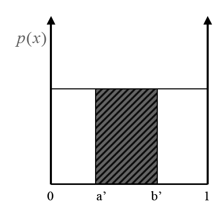
uniformly distributed random variable

• \(p\) is the same everywhere in the interval
  • \(p(x) = \text{const}\) and \(\int_a^b p(x)dx = 1\) implies

\[p(x) = \frac{1}{b-a}\]

expected value and variance

• expected value: \(E[x] = \int_a^b xp(x) dx\)
  • \(E[g(x)] = \int_a^b g(x)p(x)dx\)
• variance: \(\sigma^2[x] = \int_a^b (x-E[x])^2 p(x) dx\)
  • \(\sigma^2[g(x)] = \int_a^b (g(x)-E[g(x)])^2 p(x)dx\)
• estimating expected values: \(E[g(x)] \approx \frac{1}{N} \sum_{i=1}^N g(x_i)\)

multidimensional random variables

• everything works fine in multiple dimensions
  • but it is often hard to precisely define domain
    • except in simple cases

\[E[g(\mathbf{x})] = \int_{\mathbf{x} \in D} g(\mathbf{x}) p(\mathbf{x}) dA_\mathbf{x}\]

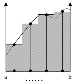
deterministic numerical integration

• split domain in set of fixed segments
• sum function values times size of segments

\[I = \int_a^b f(x)dx \qquad\qquad I \approx \sum_j f(x_j) \Delta x\]

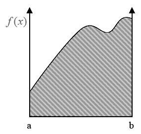
monte carlo numerical integration

• need to evaluate: \(I = \int_a^b f(x) dx\)
• by definition: \(E[g(x)] = \int_a^b g(x) p(x) dx\)
• can be estimated as: \(E[g(x)] \approx \frac{1}{N} \sum_{i=1}^N g(x_i)\)
• by substitution: \(g(x) = f(x)/p(x)\)

\[I = \int_a^b \frac{f(x)}{p(x)} p(x)dx \approx \frac{1}{N} \sum_{i=1}^N \frac{f(x_i)}{p(x_i)}\]

monte carlo numerical integration

intuition: compute the area randomly and average the results

\[I = \int_a^b f(x) dx \qquad\qquad I \approx \bar{I} = \frac{1}{N} \sum_{i=1}^N \frac{f(x_i)}{p(x_i)}\]

monte carlo numerical integration

formally, we can prove that

\[\bar{I} = \frac{1}{N} \sum_{i=1}^N \frac{f(x_i)}{p(x_i)} \quad\Rightarrow\quad E[\bar{I}] = E[g(x)]\]

meaning that if we were to try multiple times to evaluate the integral using our new procedure, we would get, on average, the same result

variance of the estimate: \(\sigma^2[\bar{I}] = \frac{1}{N} \sigma^2[g(x)]\)

example: integral of constant function

analytic integration

\[I = \int_a^b f(x)dx = \int_a^b kdx = k(b-a)\]

monte carlo integration

\[\begin{array}{rl} I & = \int_a^b f(x) dx = \int_a^b k dx \approx \\ & \approx \frac{1}{N} \sum_{i=1}^N \frac{f(x_i)}{p(x_i)} = \frac{1}{N} \sum_{i=1}^N k(b-a) = \\ & = \frac{N}{N} k(b-a) = k(b-a) \end{array}\]

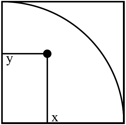
example: computing \(\pi\)

take the square \([0,1]^2\) with a quarter-circle in it

\[\begin{array}{rcl} A_{\mathit{qcircle}} & = & \int_0^1 \int_0^1 f(x,y) dx dx \\ f(x,y) & = & \begin{cases} 1 & (x,y) \in \mathit{qcircle} \\ 0 & \text{otherwise} \end{cases} \end{array}\]

example: computing \(\pi\)

estimate area of quarter-circle by tossing point in the plane and evaluating \(f\)

\[A_\mathit{qcircle} \approx \frac{1}{N} \sum_{i=1}^N f(x_i, y_i)\]

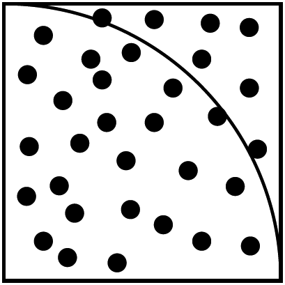
example: computing \(\pi\)

• by definition: \(A_\mathit{qcircle} = \pi / 4\)
• numerical estimation of \(\pi\)
  • without any trig functions

\[\pi \approx \frac{4}{N} \sum_{i=1}^N f(x_i,y_i)\]

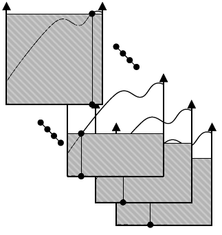
monte carlo numerical integration

• works in any dimension!
  • need to carefully pick the points
  • need to properly define the pdf
    • hard for complex domain shapes
    • e.g., how to uniformly sample a sphere?
• works for badly-behaving functions!

\[ I = \int_{\mathbf{x} \in D} f(\mathbf{x}) dA_\mathbf{x} \approx \frac{1}{N} \sum_{i=1}^N \frac{f(\mathbf{x})}{p(\mathbf{x})}\]

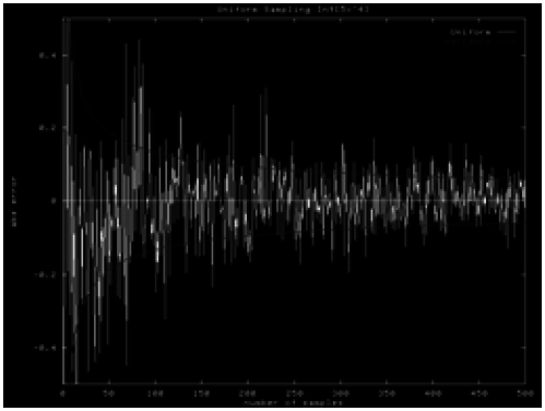
monte carlo numerical integration

• expected value of the error is \(O(1/\sqrt{N})\)
  • convergence does not depend on dimensionality
  • deterministic integration is hard in high dimensions